Evolving cellular automata to solve problems, part 1
Recently I finished reading Complexity: A Guided Tour, by Melanie Mitchell, which reminded me a lot of Gödel, Escher Bach (indeed, the book is dedicated to Douglas Hofstadter). It has reminded me that emergence is an incredibly fascinating concept – simple individual units somehow coming together to result in complex behaviour that cannot really be explained in terms of the components. In this post, we analyse the emergent behaviour of a cellular automaton and attempt to use it to solve a simple problem.
One of the first examples of emergence discussed in the book is the army ant: even in groups of 100, these ants are completely useless and will walk in circles until they die of exhaustion. But in a colony, they show remarkable sophistication and a “superintelligence”. I would highly recommend the article Army Ants: a Collective Intelligence, by Nigel Franks, and this short David Attenborough clip for more information. Apart from ants, Mitchell also makes consistent reference to cellular automata, the study of which really led to the growth of complexity science as a distinct field.
Cellular automata (CAs) have managed to divert the attention of many great scientists – Stephen Wolfram considers them the foundation of a “new kind of science”. I am clearly not one of these great thinkers, because I have never really understood what the fuss is all about. Although I have written about Conway’s Game of Life (a special case of CAs) in a previous post), I admit that I was more interested in the implementation than in the CAs.
But Complexity has given me a fascinating new perspective. In Chapter 11, Mitchell introduces the idea that CAs can be designed (or should I say evolved) to solve computational tasks. Although it is widely known that the Game of Life is Turing-complete (arguably more interesting than Mitchell’s idea), this always felt far too abstract for me to appreciate – the proof relies on a demonstration that some logic gates can be emulated, rather than actually constructing a nontrivial program. However, in Evolving Cellular Automata with Genetic Algorithms (the journal article on which Chapter 11 is based), Mitchell and coauthors tangibly demonstrate that genetic algorithms can be used to evolve a CA to perform a simple but nontrivial task.
The paper is very interesting, but does not come with source code (in their defense, it was written in 1996 and they refer to the internet as the “World Wide Web”). I think that their work deserves a modern recreation and analysis, with the benefit of intuitive code in python and more processing power.
Because this is quite a large topic, I will split it into two parts. Today’s post will set up the problem, dealing with notation and terminology, as well as discussing the nature of the CAs considered. We will leave it to a future post to actually apply genetic algorithms to evolve CAs.
Contents
- A quick introduction to cellular automata
- Computation with cellular automata
- The majority ruleset
- Conclusion
A quick introduction to cellular automata
A cellular automaton can be thought of as a set of units (cells) whose states change based on simple rules. In the Game of Life, the universe is a 2D grid of binary cells (either alive or dead), with the update rules as follows:
- A living cell (black) will die if it has fewer than two live neighbours or more than three live neighbours – roughly corresponding to underpopulation and overpopulation respectively
- A dead cell (white) will come alive if it has exactly three living neighbours (captures the idea of reproduction).
Note that to begin applying the rules, some initial condition must be specified – in practice, small changes in this starting point can drastically affect the resulting behaviour.
For our purposes we will be dealing with an arguably simpler model: a 1D binary CA. In this case, the universe consists of a row of N cells, each of which can either be dead (0) or alive (1), and is updated by looking at the radius R of surrounding cells. So if $R=3$, any update rules must map a 7-bit input (the 3 cells on either side, and the cell itself) to a 1-bit output (whether the cell will be dead or alive). A given rule might look something like this, bearing in mind that the output bit determines the new state of the middle cell:
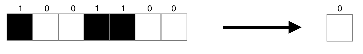
A ruleset is the set of mappings between all possible input configurations and their output states. We may as well begin to speak in specific terms referring to $R=3$, in which case a ruleset is a mapping between all possible 7-bit binary strings to a binary output:
| Input | Output |
|---|---|
| 0000001 | 1 |
| 0000010 | 0 |
| … | … |
| 0100101 | 0 |
| 0100110 | 1 |
| … | … |
| 1111110 | 1 |
| 1111111 | 0 |
If we assume that the input is ordered, then as a convenience of notation we can say that a ruleset is equal to the binary string formed by concatenating the output bits – in the above example, this is $10…01…10$.
It is very important to be comfortable with this concept: we are representing rulesets with binary strings of length 128, because there are 128 possible 7-bit inputs. Later on, we will also be using binary numbers to represent configurations of cells, so please remember to distinguish the two.
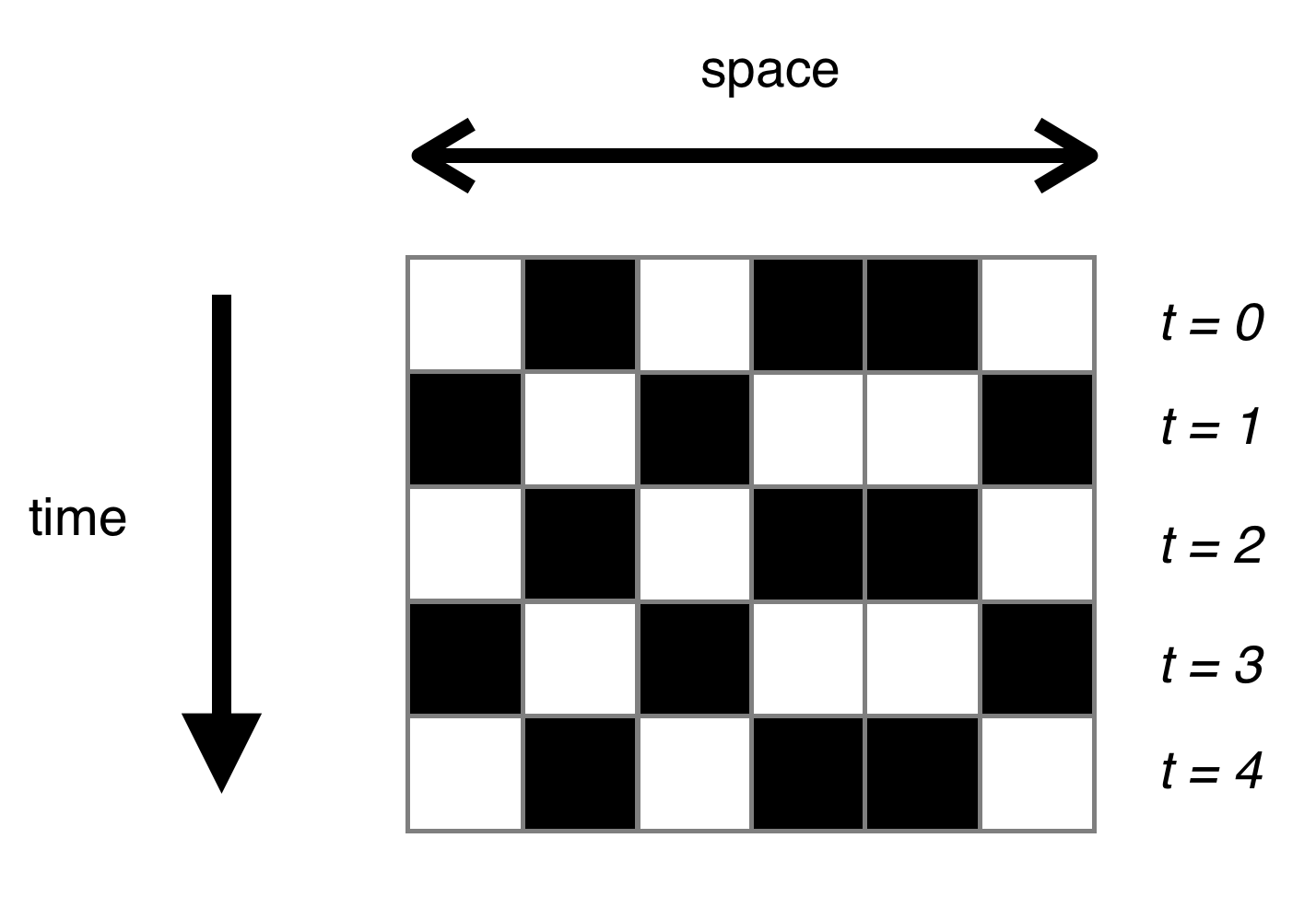
Because we are dealing with long 1D universes, animation is probably not the visualisation tool of choice (though it works very nicely for 2D). Instead, we will use a space-time diagram, which essentially stacks the generations on top of each other (with time going down the page). Here’s an example, with a simple rule that switches input bits:
Computation
I am going to conveniently sidestep the issue of properly defining “computation”. As far as this post is concerned, computation is what a computer does – a CA “computes” if it solves some task for a variable input. I would refer you to Complexity if you’d like a meaningful discussion.
The paper’s main objective is the density classification task, in which the CA must decide whether the ‘density’ of 1s in the initial configuration is greater than some cutoff proportion. Because density is typically denoted by $\rho$, this is more precisely referred to as the $\rho_c = 1/2$ task.
To put it simply, the CA must decide whether the initial setup had more living or dead cells (1s or 0s). If there were more 1s, then after some number of iterations, we want the CA to display all 1s. Otherwise, if there were more 0s, we want the CA to display all 0s. An example mapping is shown below:
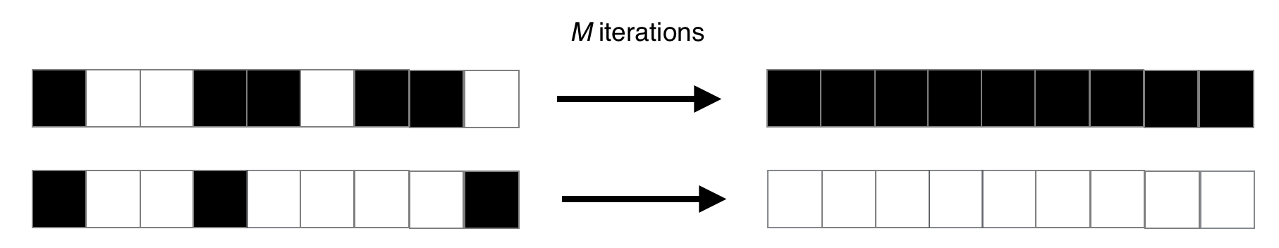
You may be questioning the difficulty of that task. After all, it’s as easy as iterating over the universe and counting the number of 1s, then determining the output based on this value! But remember the catch: each cell only has access to a fixed neighbourhood of three cells on either side. There is nowhere we can store the count: each cell can only make a decision based on its neighbours and change its state accordingly.
The majority ruleset
Before we bother with genetic algorithms, it is worth checking how a simple solution performs. For this, we will use the majority ruleset, in which each cell will just change its state to match the majority of its 7-cell neighbourhood.
Although it is conceptually straightforward, it is at this stage that we need to consider the details of the implementation in python. We will be using strings of binary digits to store configurations; they are efficient and easy to work with. At a high level, we need to do the following:
- generate the majority ruleset (of course we are not going to hard code all 128 rules)
- generate a random initial configuration (i.e a random binary number)
- iterate the initial configuration according to the majority ruleset
- plot the space-time diagram
Here are some of the global constants that we need for now, though we will introduce many more when we get onto genetic algorithms:
R = 3  # size of neighbourhood
N_RULES = 2 ** (2 * R + 1)  #  number of rules in a ruleset
N = 79  # number of cells in universe
The number of rules is $2^7 = 128$ (the number of possible 7-bit inputs). Incidentally, this means that the number of possible rulesets is $2^{128}$ – a clear indication that we will not be able to find a solution by brute force.
Generating the majority ruleset
We are going to treat rulesets as python dictionaries. This is quite natural, since a ruleset is essentially a bijective mapping between all possible 7-bit inputs (keys) and the output bits (values). We will generate the keys and values separately.
def rule_keys(n_rules, radius=3):
    rule_input = []
    for i in range(n_rules):
        binary = str(bin(i))[2:].zfill(2*radius + 1)
        rule_input.append(binary)
    return rule_input
This could also be refactored into a one-line generator expression:
rule_keys = (str(bin(i))[2:].zfill(7) for i in range(N_RULES))
But out of respect for Guido I have kept it as a function with a loop inside (which is slightly faster anyway). The [2:] is used to slice away the ugly 0b that python prepends to a binary number, and zfill pads the string with leading zeroes.
To complete the majority ruleset, we just need to know if there are more 1s or 0s in the input. We will use a bit of python trickery to make this more concise:
majority_ruleset = {}
for rule_input in rule_keys(N_RULES):
    # 1 if the majority of the neighbourhood is 1.
    out = int((sum(d == "1" for d in rule_input) > R))
    majority_ruleset.update({rule_input: str(out)})
The statement (sum(d == "1" for d in rule_input) > R is True if there are more than 3 living cells in the input (remember that R = 3), and False otherwise. We then cast this to an int (1 or 0) then a str (“1” or “0”), and update the ruleset with this key-value pair. This is an excerpt from the resulting ruleset:
 {
     '1010010': '0',
     '1010011': '1',
     '1010100': '0',
     '1010101': '1',
     '1010110': '1',
     '1010111': '1',
     '1011000': '0',
     '1011001': '1',
 }
Generating a random initial configuration
One might think that the best way to generate a random configuration is just to combine N random bits where N is the size of the universe. However, consider the density of 1s in such a configuration – it is a (literal) textbook example of a binomial distribution with $\rho \sim B(N, 0.5)$.
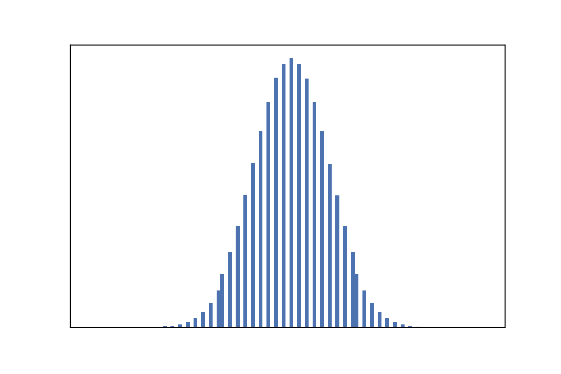
Notice the strong peak at 0.5, meaning that most of the initial configurations will have a roughly equal split of 0s and 1s. This is not ideal for us to explore the density classification task, because we do want to have enough easy cases (i.e clear majorities).
As such, we will adopt a slightly different strategy:
- Randomly choose a density of 1s that we want in the configuration (sampled from a uniform distribution).
- Form an ordered universe with that number of 1s, and the rest 0s
- Shuffle the universe
A small snippet that does this is as follows:
n_ones = random.randrange(0, N)
binary = "1" * n_ones + "0" * (N - n_ones)
result = "".join(random.sample(binary, N))
We could use random.shuffle() in the third line, but that works in-place (and requires a list), so the chosen solution is cleaner. In the end, I decided to generalise the above slightly, letting you change the range of the uniform sample and specify the length of the output string:
def uniform_random_binary(length, lower=0, upper=None):
    # The defualt upper bound is the length
    if upper is None:
        upper = length
    n_ones = random.randrange(lower, upper)
    binary = "1" * n_ones + "0" * (length - n_ones)
    return "".join(random.sample(binary, length))
Iterating an automaton
To remain general, our iteration function should take in a configuration, a ruleset, and a radius. One iteration consists of applying the appropriate rule to each bit in the universe’s configuration, which is done by getting a cell’s neighbours as a 7-bit binary string, then using the ruleset dictionary to find the output bit.
def single_iteration(config, ruleset, radius):
    next_iteration = ""
    # Support wrapping by extending either end
    extended_config = config[-radius:] + config + config[:radius]
    for i in range(radius, len(config) + radius):
        neighbours = extended_config[i-radius:i+radius+1]
        next_iteration += ruleset[neighbours]
    return next_iteration
The complexity in the above implementation arises because we need a circular universe, so we must extend the configuration to allow for ‘wrapping’.
To iterate multiple times, we repeatedly apply the single_iteration() function:
def iterate_automata(initial, ruleset, n_iter, radius=3,
                     verbose=False):
    config = initial
    history = [config]
    for _ in range(n_iter):
        config = single_iteration(config, ruleset, radius)
        if verbose:
            print(config)
        history.append(config)
    return history
This function also keeps track of the CAs history, which is necessary if we want to use a space-time diagram for visualisation.
Space-time diagrams
If we run iterate_automata() with verbose=True, it’ll print the universe at each time step, so in a sense that is a space-time diagram. However, it is fair to ask for something more stylish, for which we will use matplotlib’s imshow:
def plot_spacetime_diagram(binary_history, filename=None):
    arr = np.array([[int(digit) for digit in row]
                     for row in binary_history])
    plt.figure()
    plt.imshow(arr, cmap="Purples_r")
    if filename is None:
        plt.show()
    else:
        plt.savefig(filename)
Tying it together
Now that we have implemented the pieces, testing the majority ruleset is very simple:
random.seed(0)
initial_config = uniform_random_binary(N)
majority_history = iterate_automata(initial_config,
                                    majority_ruleset,
                                    n_iter=N,
                                    radius=R)
plot_spacetime_diagram(majority_history)
Looking at the space-time diagrams for different random seeds shows that in general, the majority ruleset does not consistently solve the $\rho_c = 1/2$ task:
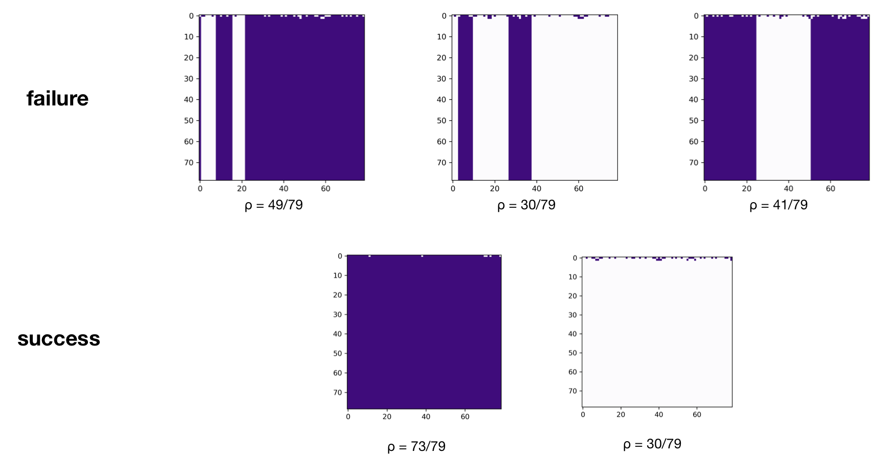
The above results are very similar to what Mitchell et al. found (though they use $N = 149$), which gives us a good indication that our implementation thus far has been accurate.

Conclusion
In this post, we have laid the framework for using cellular automata to solve a computational task, namely, classifying the density of living cells in the initial conditions.
We have examined the failings of a ‘local’ solution that naively treats a cell’s immediate neighbourhood as a proxy for the entire universe, and thus see the need for emergent computation, in which individual cells somehow learn to appreciate the rest of the universe and come up with a global solution.
In the next post, we discuss how genetic algorithms can be applied to evolve the cellular automata to solve the density classification task, rather than having to supply a hand-crafted rule, or do a brute force search over all possible rulesets (which we have shown to be infeasible). Stay tuned.