The Leibniz integral rule in electrodynamics

I have been slowly working through David Griffith’s widely-used textbook, Introduction to Electrodynamics. It is known for having a large number of reasonably difficult exercises, which are instrumental in conveying some concepts not directly addressed in the main text. I found an elegant shortcut to one of the questions, which was not noted in the solution manual. The shortcut involves (ab)using a very versatile, if slightly overlooked theorem in calculus – the Leibniz integral rule. I will briefly discuss this, before working through the problem.

The Leibniz integral rule

The Leibniz rule concerns derivatives of integrals; the most basic form is as follows:

\[\frac{d}{dx} \left( \int_a^b f(x,t) dt \right) = \int_a^b \frac{\partial}{\partial x} f(x,t) dt\]

This can be proven by letting $I(x) = \int_a^b f(x,t) dt$, then using the definition of the derivative to evaluate $I’(x)$, which will be left as an exercise for the reader. However I hope you can get an intuitive feel for this: the integral measures the total variation with respect to $t$, whereas the derivative measures the rate of change with respect to $x$, so it makes sense that the order of operation doesn’t really matter.

A slightly more general version concerns the case where the limits of the integral are variable:

\[\frac{d}{dx} \left( \int_{a(x)}^{b(x)} f(x,t) dt \right) = f\left(x, b(x)\right)\frac{d b(x)}{dx} - f(x, a(x))\frac{d a(x)}{dx} + \int_{a(x)}^{b(x)}\frac{\partial}{\partial x} f(x,t) dt\]

Effectively, it is the same as what we had before, plus some additions to take into account of the variable limits. This formula can be explained in terms of the fundamental theorem of calculus, but the derivation is besides the point. For now, I would urge you to just accept the above rule (it is surprisingly useful). Let’s go through an example to evaluate the following expression:

\[\frac{d}{dx} \int_{\sin x}^{\tan x} \sqrt{1+ t^3}dt\]

Hint: do not do it by evaluating the indefinite integral, substituting in the limits, then differentiating. Applying the Leibniz rule, we see that:

\[\begin{aligned} \frac{d}{dx} \int_{\sin x}^{\tan x} \sqrt{1+ t^3}dt &= \sqrt{1+ \tan^3 x}\frac{d}{dx}\tan x - \sqrt{1 + \sin^3 x} \frac{d}{dx} \sin x\\ &= \sec^2x\sqrt{1+ \tan^3 x} - \cos x \sqrt{1 + \sin^3 x} \end{aligned}\]

The electrodynamics problem

I say ‘electrodynamics’, but really it is an electrostatics problem. Below I have reproduced the question from Chapter 2 (Electrostatics) of Griffith’s Introduction to Electrodynamics. It has been edited slightly.

Problem 27 Find the electric field on the axis of a uniformly charged solid cylinder, at a distance z from the centre. The length of the cylinder is L, its radius is R, and the charge density is $\rho$.

Our general strategy will be to first find the potential (or rather, an expression for the potential), by decomposing the cylinder into simpler shapes. Then we will find the field using $\mathbf{E} = - \nabla V$.

A cylinder can be thought of as many discs; a disc can be thought of as many rings; a ring can be thought of as many point charges. We will thus build a cylinder.

1. A single point charge

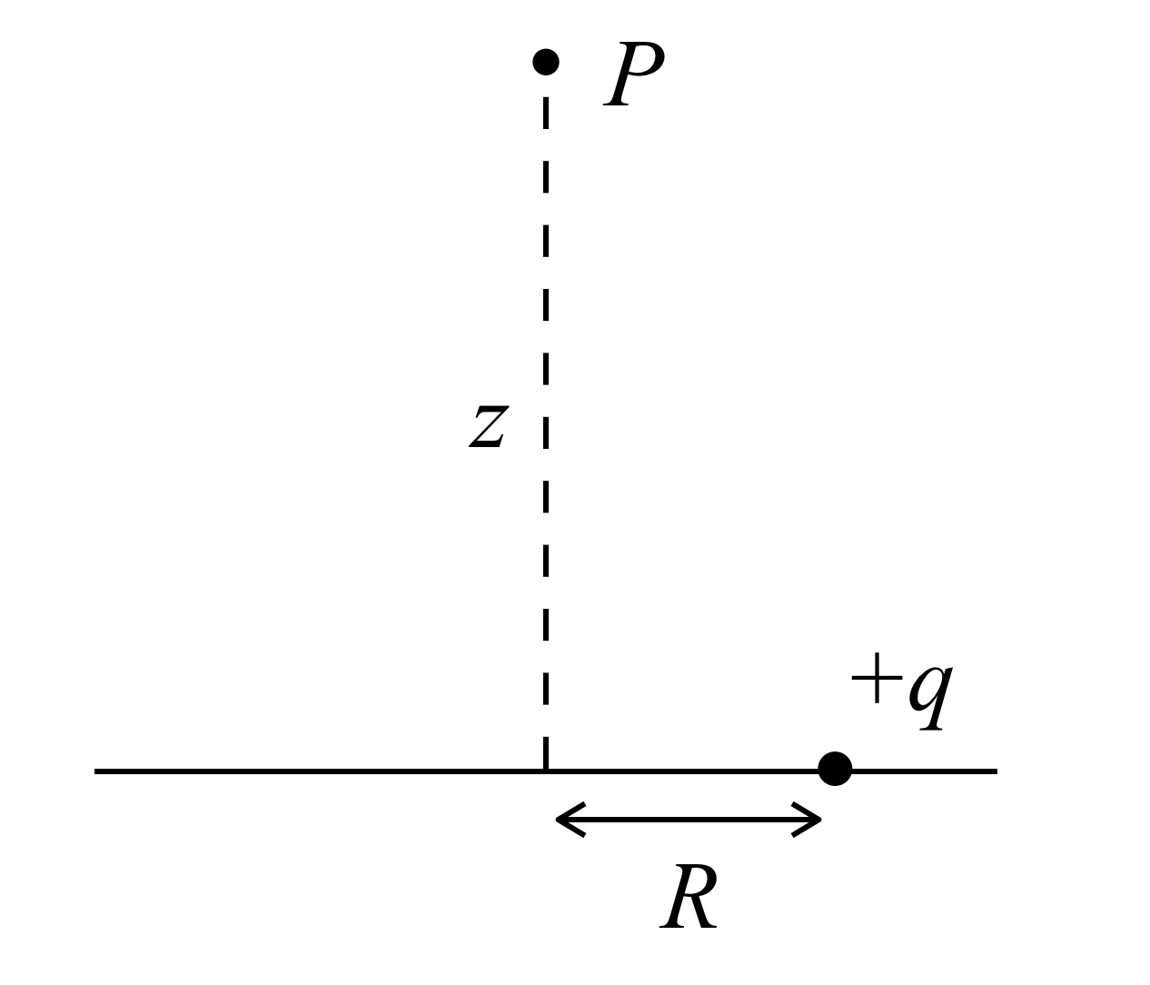
Recall the formula for the potential at a point $P$:

\[V = \frac{1}{4\pi \epsilon_0} \frac{q}{r}\]

In this formula, $r$ is the displacement between the charge and the test point. Applying Pythagoras’ theorem to the diagram, we see that $r^2 = R^2 + z^2$.

Plugging values into the formula:

\[V = \frac{1}{4\pi \epsilon_0} \frac{q}{\sqrt{R^2 + z^2}}\]

2. A ring of charge

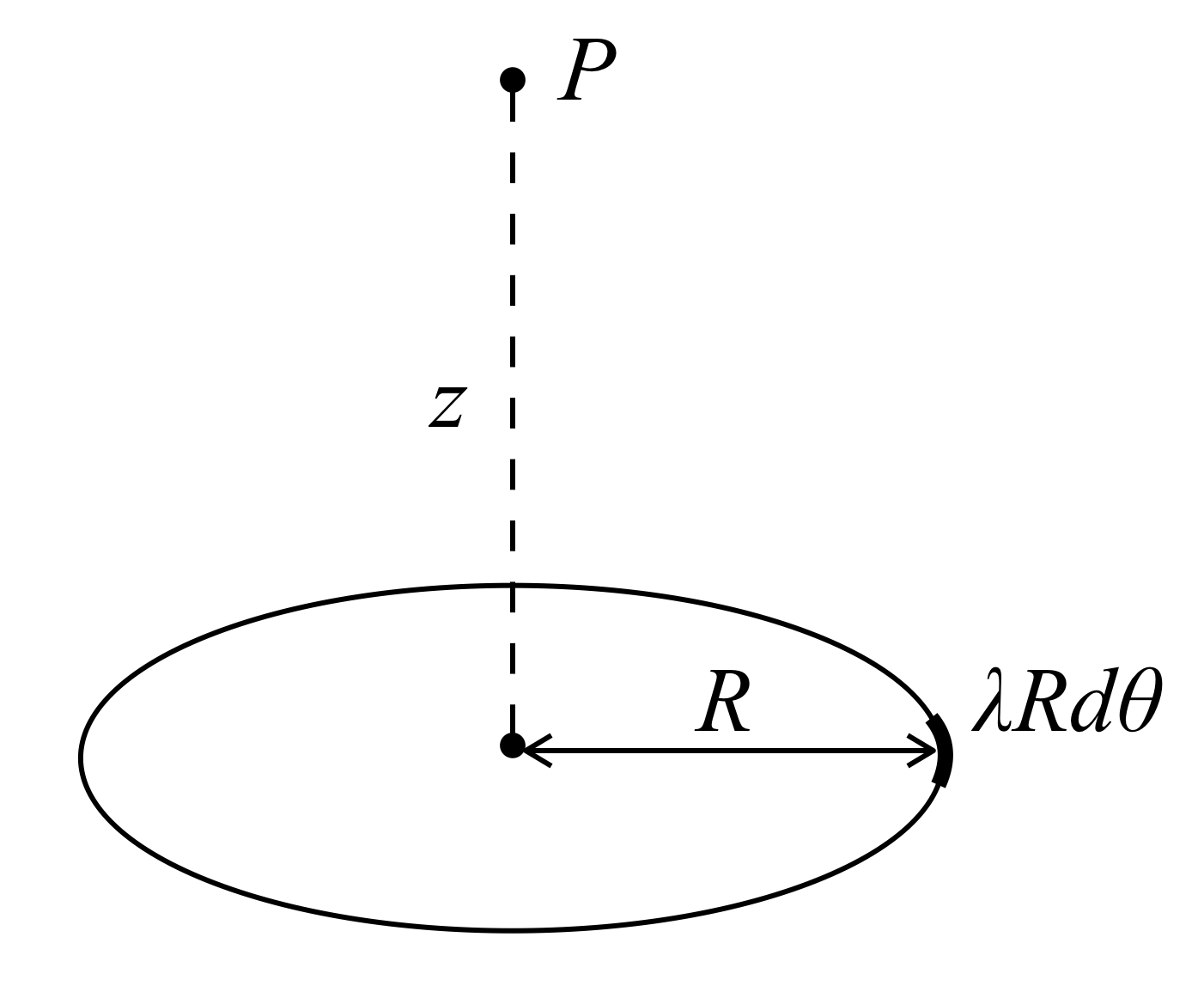
In order to find the potential for a ring of charge given the potential of a point charge, we consider a charge element $\lambda dl$. But the length of a segment on a circle is given by $R \theta$, so we can say that $dl = R d\theta$.

Instead of a positive point charge $q$, we now have a charge element $\lambda R d\theta$. Using our previous result, the potential at P from one of these charge elements is:

\[dV = \frac{1}{4\pi \epsilon_0} \frac{\lambda R d\theta}{\sqrt{R^2 + z^2}}\]

The total potential for the ring is the sum of the contributions from each of the charge elements.

\[V = \int_0^{2\pi} \frac{1}{4\pi \epsilon_0} \frac{\lambda R d\theta}{\sqrt{R^2 + z^2}} = \frac{1}{4\pi \epsilon_0} \frac{\lambda R }{\sqrt{R^2 + z^2}} \int_0^{2\pi} d\theta\] \[\therefore V = \frac{1}{4\pi \epsilon_0} \frac{2 \pi R \lambda}{\sqrt{R^2 + z^2}}\]

3. A disc of charge

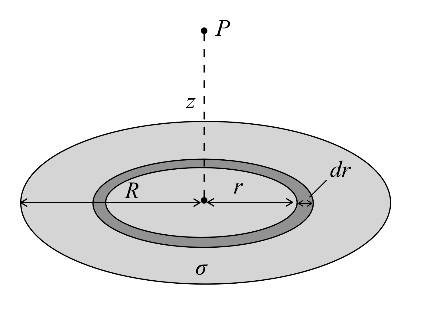
We can build up a disc of charge with radius R from an infinite number of rings of charge of radius r. Note that this r is different to the one briefly mentioned earlier, which was the separation between P and the charge.

Because we are going from 1D to 2D, we must let $\lambda = \sigma dr$, where $\sigma$ is the surface charge. Thus the potential from one ring is:

\[dV = \frac{1}{4\pi \epsilon_0} \frac{2 \pi r \sigma dr}{\sqrt{r^2 + z^2}}\]

We could arrive at this otherwise, by noting that the total charge in the ring is

\[\sigma \cdot \text{area} = \sigma \cdot 2\pi r dr\]

Anyway, let us continue.

\[V = \frac{\sigma}{2 \epsilon_0} \int_0^R \frac{r}{\sqrt{r^2 + z^2}} dr\]

As is rarely the case in electrodynamics, this integral is not at all difficult to evaluate. We use the ‘reverse chain rule’ to see that:

\[\int_0^R \frac{r}{\sqrt{r^2 + z^2}} dr = \int_0^R r \left( r^2 + z^2\right)^{-1/2} dr =\left[ (r^2+z^2)^{1/2} \right]_0^R\]

The total potential is then easily found.

\[V = \frac{\sigma}{2\epsilon_0} \left(\sqrt{R^2+z^2} - z \right)\]

4. A cylinder of charge

We are now ready to tackle the original problem. Here it is again:

Find the electric field on the axis of a uniformly charged solid cylinder, at a distance z from the centre. The length of the cylinder is L, its radius is R, and the charge density is $\rho$.

I’ll set up the solution in the same way Griffiths does – this image is taken from the solution manual.

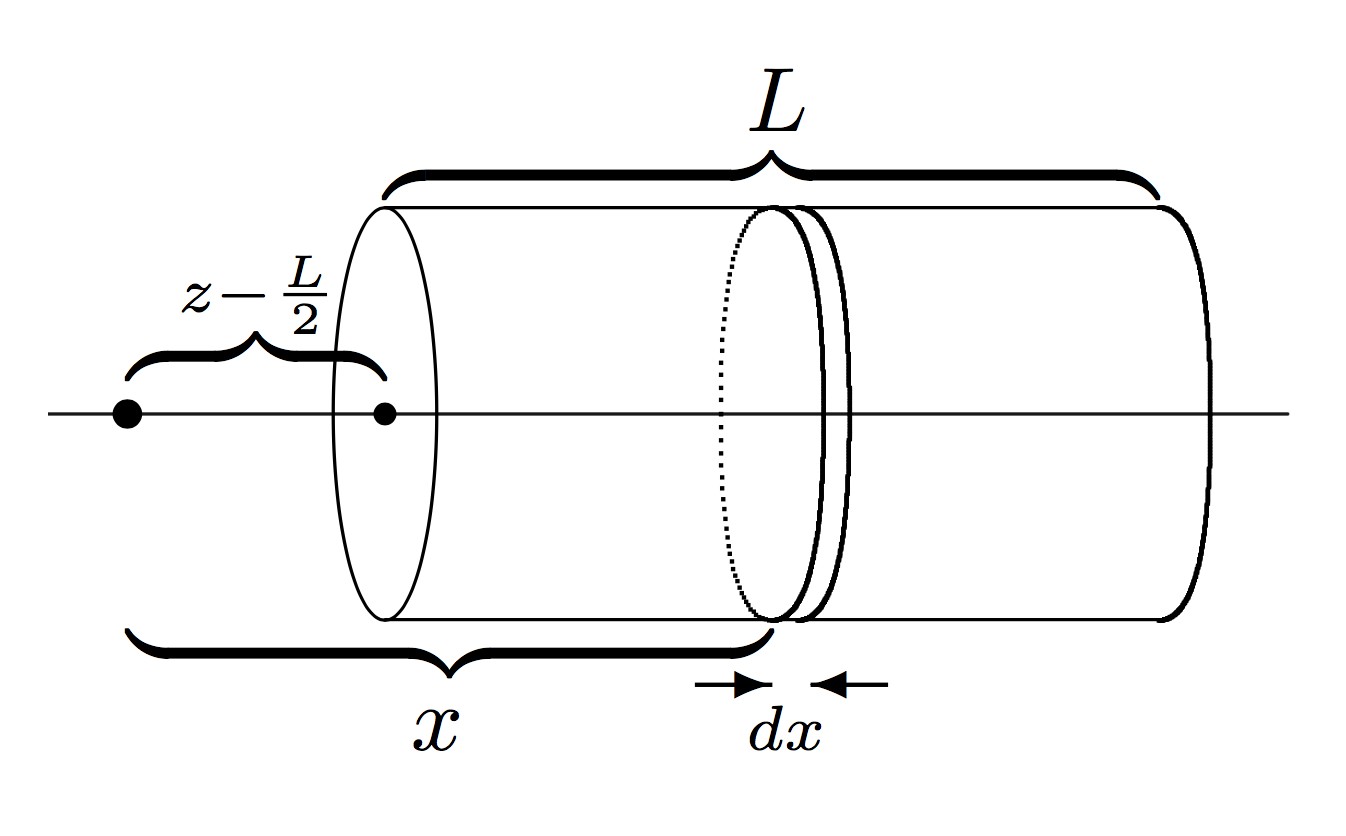
A cylinder is made up of an infinite number of discs. We want an expression for the potential at the test point, a distance z from the centre. We will let x denote the distance between the test point and a given disc. The potential from one such disc is given by the formula we found earlier, with the substitution $z \rightarrow x$ and $\sigma \rightarrow \rho dx$:

\[dV = \frac{\rho dx}{2 \epsilon_0} \left( \sqrt{R^2 + x^2} - x \right)\]

Since L is the length of the cylinder, and z is the distance from the centre of the cylinder, it is clear that there are discs all the way from $x = z - \frac L 2$ to $x = z+ \frac L 2$. The total potential at our test point is just the integral over all of these discs:

\[V = \frac{\rho}{2\epsilon_0} \int_{z-L/2}^{z+L/2}(\sqrt{R^2 + x^2} - x) dx\]

Despite the simple-looking expression, this integral will soon become a nightmare to evaluate. And don’t forget – we are trying to find the electric field, so we will then have to take the gradient of the whole mess.

To be clear, because of the cylinder’s symmetry, ‘taking the gradient’ here just means differentiating with respect to z, but nevertheless this will not be a fun calculation.

\[\mathbf{E} = - \nabla V = - \mathbf{\hat{z}} \frac{\partial V}{\partial z}\]

Leibniz to the rescue

Instead of immediately evaluating the integral to calculate the potential, then differentiating, why don’t we write it in one expression first:

\[\mathbf{E} = - \mathbf{\hat{z}} \frac{\rho}{2\epsilon_0} \frac{\partial}{\partial z} \int_{z-L/2}^{z+L/2}\left( \sqrt{R^2 + x^2} - x \right) dx\]

This might look more complicated, but in fact it makes life much easier. Because we are taking the derivative of an integral, we can simply apply the Leibniz integral rule. The limits are not constant, but the integrand is independent of z, so the rule tells us that:

\[\begin{align*} \mathbf{E} = - \mathbf{\hat{z}} \frac{\rho}{2\epsilon_0} &\bigg[ \left( \sqrt{R^2 + (z+L/2)^2} - (z+L/2) \right) \frac{\partial}{\partial z}(z+L/2)\\ & - \left( \sqrt{R^2 + (z-L/2)^2} - (z-L/2) \right) \frac{\partial}{\partial z}(z-L/2) \bigg] \end{align*}\]

Intuitively, there is some kind of ‘cancellation’ between the differentiation and integration, so we simply substitute the limits into the integrand (and multiply by the derivative of the limit since it is not constant), then subtract. In this case it is even simpler because the derivatives of the limits are unity:

\[\mathbf{E} = \frac{\rho}{2\epsilon_0} \left[L + \sqrt{R^2 + (z-L/2)^2} - \sqrt{R^2 + (z+L/2)^2} \right] \mathbf{\hat{z}}\]

Conclusion

In many electrodynamics problems, one finds the electric field by first calculating the potential, then taking the gradient. I hope I’ve given you a reasonable motivation to not just do this mechanically – keep an eye out for shortcuts that will save you time, and reduce the chances of you making a minor algebraic error.