Evolving cellular automata to solve problems, part 2
We will be picking up where the previous post left off. As a brief summary, we are attempting to replicate the results of Evolving Cellular Automata with Genetic Algorithms (Mitchell, Crutchfield and Das 1996), dealing with the density classification task for 1D binary cellular automata (CAs). To put it simply, we are trying to design a ruleset such that the final configuration of a cellular automaton after M iterations is either all 1s or all 0s depending on which class was more common in the initial state. The caveat is that each cell in the universe can only make its decision based on the three neighbours to the left and right.
We examined the failures of the majority ruleset, an ‘obvious’ solution in which each cell updates to the local majority among its neighbourhood, and thus see the need for something more sophisticated. At the same time, we saw that the space of possible solutions is in the order of $10^{38}$, meaning that any kind of brute force method will not be feasible. This invites the use of genetic algorithms (GAs), with which we could evolve a CA to perform this task without ever explicitly devising a ruleset.
Genetic algorithms in the context of CAs
A complete treatment of genetic algorithms is not in the scope of this post (the wikipedia page is a good start), but I will attempt to cover the salient points:
- We start with a population of different possible rulesets. This is a very important point – the individuals in the population are not the cellular automata, they are what we are trying to optimise, which in this case is the ruleset.
- Rulesets in the population have different fitnesses, corresponding to how well they solve the $\rho_c = 1/2$ task. We will define the fitness F to be the proportion of random ICs on which the ruleset succeeds (becomes all 1 or all 0 correctly). So if we test a ruleset on 100 random ICs and 35 are classified correctly, $F = 0.35$
- In each generation, we compute the fitness for each ruleset in the population. The fittest rulesets (the elites) are cloned to the next generation, but we also crossover (i.e breed) these rulesets to form offspring, which are then mutated before joining the next generation.
- Over many generations, we should see the fitness increase, as the traits of the favourable rulesets are passed onto the next generation.
The GA acts as a more efficient way to traverse the huge space of possible rulesets in search of one that can suitably solve the density classification task – it does not guarantee that the global optimum will be reached.
Implementation
For the most part, the functions used in this post are the same as in part 1, though took care to make obvious optimisations because the evolution of the CAs will involve repeated calls of the same functions.
The initial population consists of random rulesets. To generate a single random ruleset, we zip the the rule inputs (7-bit binary strings) with random 1s or 0s which are obtained from the uniform_random_binary function we defined. For convenience, we can uniquely refer to a given ruleset with a hexadecimal ID, which is made by converting the binary string of all rule outputs (assuming ordered inputs) into hexadecimal.
def random_ruleset(n_rules):
    rule_values = uniform_random_binary(n_rules)
    hex_id = hex(int(rule_values, 2))
    return hex_id, dict(zip(rule_keys(n_rules), rule_values))
To generate the initial population of 100 (or more generally, n_ic) ICs, it is not as simple as running random_ruleset 100 times because we want exactly half of the ICs to have a majority of 1s.
def generate_random_ICs(universe_size, n_ic=100):
    ics = []
    cutoff = int(0.5 * universe_size) + 1
    # Exactly half of the initial conditions will have p < 0.5
    for _ in range(n_ic // 2):
        minority = uniform_random_binary(universe_size, 0, cutoff)
        majority = uniform_random_binary(universe_size, cutoff,
                                         universe_size + 1)
        ics.append(minority).append(majority)
    return ics
Prior to implementing crossover and mutation, we will define a helper function that converts a hex ID into a ruleset, by converting the hexadecimal to binary and zipping this with a list of 7-bit rule inputs:
def hex_to_ruleset(hex_id, n_rules=128):
    rule_values = bin(int(hex_id, 16))[2:].zfill(n_rules)
    return dict(zip(rule_keys(n_rules), rule_values))
As discussed in the paper, crossover involves pointwise swaps between two parent rulesets, and mutation involves randomly switching bits.
def crossover_and_mutate(hex1, hex2, n_rules=128,
                         n_crossover_points=1, n_mutations=2):
    bin1 = list(bin(int(hex1, 16))[2:].zfill(n_rules))
    bin2 = list(bin(int(hex2, 16))[2:].zfill(n_rules))
    # Crossover: get indices of unequal, then
    # randomly select an index to swap
    unequal_indices = [i for i, digit in enumerate(bin1) if
                       bin2[i] != digit]
    if len(unequal_indices) > n_crossover_points:
        crossover_points = random.sample(unequal_indices,
                                         n_crossover_points)
        for c in crossover_points:
            bin1[c] = bin2[c]
    # Mutation
    for _ in range(n_mutations):
        idx = random.randrange(n_rules)
        # Flip bit
        bin1[idx] = str(int(not bool(bin1[idx])))
    return hex(int("".join(bin1),2))
Metaparameters
As with most optimisation methods, genetic algorithms have a number of metaparameters that can drastically change the resulting behaviour, for example the number of generations, the mutation rate, the size of the initial population of chromosomes, etc.
GEN = 50
N_CHROMOSOMES = 100  # number of rulesets in each generation
N_CROSSOVER_POINTS = 1
N_MUTATIONS = 2
In addition, we shouldn’t forget the CA parameters:
N = 59  # universe size
MAX_ITER = 100  # max number of iterations to perform the task
N_IC = 100  # number of ICs each ruleset is tested on
N_RULES = 128  # number of rules in each ruleset
These are mostly similar to the choices of Mitchell et al., though I have opted for fewer generations and a much smaller universe (they use 100 and 149 respectively), which should be faster to compute and serve as a proof-of-concept.
It is important to note that genetic algorithms can be quite sensitive to initial conditions, which is why we will parameterise each run by a random seed.
Evolution
We are now ready to implement the actual genetic algorithm. The first thing to do is to set the random seed and generate the initial population. We will use a dictionary, with the keys being hex IDs and values being the rulesets.
random.seed(0)
population = {}
for _ in range(N_CHROMOSOMES):
    id, ruleset = random_ruleset(N_RULES)
    population[id] = ruleset
In each generation, we will first compute the fitness of each ruleset on 100 random ICs:
generation_ics = generate_random_ICs(N, N_IC)
fitness_log = []

for hex_id, chromosome in population.items():
    # Evaluate performance on random ICs.
    fitness = 0
    for config in generation_ics:
        # Count the majority
        majority = config.count("1") > len(config) // 2
        # Iterate automaton
        hist = iterate_automata(config, chromosome, MAX_ITER,
                                verbose=False)
        # If the CA has classified correctly, increment fitness
        if hist[-1] == str(int(majority)) * len(config):
            fitness += 1
    print("hex_id", hex_id, "  Fitness", fitness)
    fitness_log.append((hex_id, fitness))
Next, we determine who are the elites (the top 20 rulesets):
# Find top 20 in population
fitness_log.sort(key=lambda x: x[1], reverse=True)
elites = [i[0] for i in fitness_log[:20]]
print("Generation best:", fitness_log[0])
print("Least fit elite:", fitness_log[20])
As suggested by the paper, we will copy these elites directly to the next generation, then form the rest of the population by breeding these elites with replacement.
# Copy the top 20 to the next generation
new_population = {}
for i in elites:
    new_population[i] = hex_to_ruleset(i)

# Crossover and mutate random pairs of elites
for _ in range(N_CHROMOSOMES - 20):
    parent1, parent2 = random.sample(elites, 2)
    child_hex = crossover_and_mutate(parent1, parent2,
                                     N_CROSSOVER_POINTS,
                                     N_MUTATIONS)
    new_population[child_hex] = hex_to_ruleset(child_hex)

population = new_population
We then repeat the above for many generations, and hopefully should see the fitnesses increase.
Initial observations
Judging by the success of the previous post, I was expecting the script to work immediately and yield interesting results. Alas, programming is rarely so simple. The genetic algorithm was slow (I’m used to the 5-10 seconds it takes to train most sklearn models), but what is worse, it was not able to solve the task. After 50 generations, the GA has not managed to beat random guessing:
Gen 49
==========
hex_id 0x455d652de3a5534054ed51a12093d25   Fitness 50
hex_id 0x455d652de3a5534054ec51a12093d27   Fitness 50
hex_id 0x455d652de3a5534054ed51212093d25   Fitness 50
hex_id 0x455d652de3a55b40146d51a12093d27   Fitness 50
...
Generation best: ('0x455d652de3a5534054ed51a12093d25', 50)
Least fit elite: ('0x455d652de3a55b40146d51a12093d277', 50)
A closer analysis revealed that many of the final rulesets corresponded to the naïve strategy of mapping any possible input to a 1, which results in the ruleset being correct about 50% of the time.
It should be noted that Mitchell et al. trained their genetic algorithm across 300 different runs, so it could be the case that this was one of the unlucky runs in which the GA fails to learn. But testing multiple random seeds yielded no further improvements.
A possible fix
I hypothesised that the initial population contained too many rulesets that had a clear majority of 1s or 0s, disproportionately mapping their input to one of the two regardless of the IC. Remember that this was by design, we chose to sample rulesets and ICs from a distribution uniform over the density of 1s rather than the unbiased distribution which is binomial over the density of 1s. In light of the poor empirical results, I modified the random_ruleset function to use the unbiased distribution instead:
def random_ruleset2(n_rules):
    random_binary = bin(random.randint(0, 2**n_rules - 1))
    rule_values = str(random_binary)[2:].zfill(n_rules)
    hex_id = hex(int(rule_values, 2))
    return hex_id, dict(zip(rule_keys(n_rules), rule_values))
Because it seemed that I would have to test multiple parameters, I also refactored the GA script into a function:
evolve_automata(59, n_crossover_points=1, n_mutations=6,
                random_seed=0, n_ic=100, n_gen=50,
                ruleset_generator=2)
Using this new ruleset generator, we are much less likely to have naïve outputs of all 1s or all 0s. My guess was that although this would result in the GA starting with poorer fitnesses, they would not get ‘stuck’ with naïve random-guessing strategies. However, testing revealed that fitness still converged to 50%, just at a much slower rate.
To combat this, I reasoned that the simplest way to escape local optima is to pump up the mutation rate in the hope that elites will be found that beat random guessing, and these will pass on their traits to the next generation.
Finally, we achieved some progress. I noticed that the combination of a high mutation rate and an unbiased random ruleset meant that the GA didn’t always get stuck with a 50% fitness. For N_MUTATIONS = 6, tested over 20 different seeds, mean elite fitnesses in the last 10 generations were:
[83.5, 52.2, 92.6, 51.2, 51.1, 50.0, 51.5, 51.5, 51.7, 79.2,
 83.1, 51.7, 73.5, 57.2, 51.6, 51.2, 52.1, 50.0, 78.7, 82.9]
Eight of the 20 runs resulted in fitnesses beyond the 50% level, however only one of the 20 beat 90%. This falls very far short of Mitchell et al’s claim to have at least 90% fitness on all 300 of the runs, but it is certainly progress.
Interestingly, increasing N_MUTATIONS to 12 produced worse results, with the maximum mean elite fitness being 80.2 and only six of the 20 runs resulting significantly beating 50%. N_MUTATIONS=18 does even worse, with only one of the 20 beating 50%. I think this is because having many mutations reduces the impact of crossover (which is only at a single point), so we don’t get the benefits of ‘meiosis’.
Analysis of evolved CAs
We will examine one of the rulesets which achieved a fitness of above 90%. For some different initial configurations, this is what we observe:
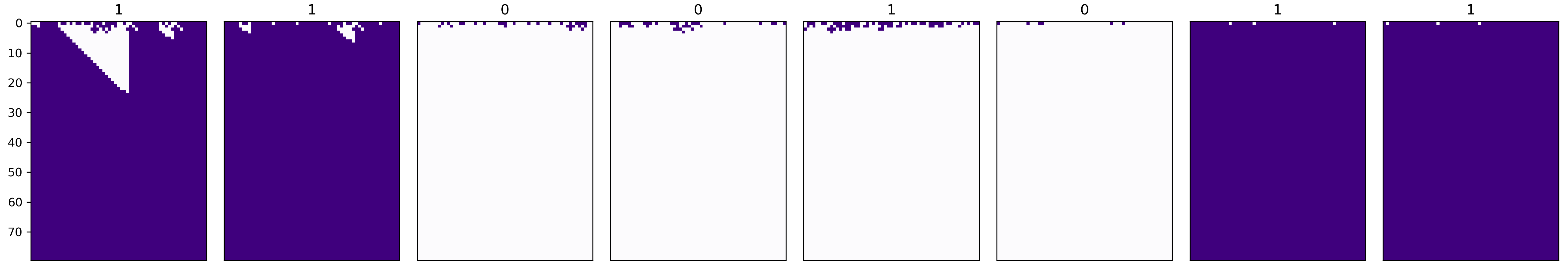
Remember that purple is alive and white is dead; I have displayed the actual majority class above each subplot. Thus the fifth subplot represents an error, because despite the majority of 1s, the final state is all 0s.
As in the paper, the ruleset works by quickly reaching a steady state of all 0s unless large blocks of 1s are found – it is not really the sophisticated emergent behaviour that I was hoping to see. The only exception is the first subplot, in which some semblance of the particle strategy is achieved.
Conclusion
Though we did achieve some interesting results, I don’t think that this exploration overall was a success. I could not replicate the results of Mitchell et al., even using a simple universe of 59 cells rather than 149. The default setup used in the paper kept getting stuck at 50% fitness, and it was only after I deviated from their suggestions that I managed to do better.
I have become somewhat disillusioned regarding the scientific value of the paper (though I still find it fascinating). The sophisticated particle strategy discovered by Mitchell et al. is remarkable, yet they seem to downplay the fact that it was observed only in a few of the 300 runs of the genetic algorithm. This is hardly reproducible, and really feels to me like grabbing at patterns in the random darkness.
Additionally, the evolution of CAs with genetic algorithms is a very slow process (I had to leave my code running over a few nights), and the results are very inconsistent. I can only imagine how long it would have taken for Mitchell et al. to conduct 300 runs with a universe size of 149 (before the turn of the millennium!). This severely limits the practical applications, and the prospect that evolved CAs could tackle more complex tasks like image processing (as suggested in the paper’s conclusion) seems chimerical.
Nevertheless, I am happy to have attempted to replicate the results, because it has been a while since I’ve played around with genetic algorithms. It was also some extra practice with python’s standard language features, of which I make extensive use. Perhaps some time in future I may realise that my implementation had a flaw and author a part 3, but for now I’m content to stay in this local optimum.
The code for this post, along with plots and data, is available as a Jupyter notebook on GitHub.