Data Structures

• Amortised analysis
• Stack ADT
• List ADT
• Queue ADT
• Dictionary ADT
• Priority queue ADT
• Disjoint Set ADT
  • Flat forest and deep forest
  • Lazy forest
• Binary Search Tree
  • BST Deletion
• 2-3-4 tree
  • 2-3-4 Insertion
• Red Black Tree
  • RBT Insertion
• B-tree
  • B-tree insertion
  • B-tree deletion
• Hash-tables
  • Chaining
  • Open addressing
• Binary heap
• Binomial heap
• Fibonacci heap
  • Analysis using potentials
  • Relationship to Fibonacci numbers

Amortised analysis

• Amortised analysis considers the average cost of a sequence of operations in a data structure.
• Aggregate analysis puts an upper bound on the total cost of n operations then states that the amortised cost is $T(n)/n$.
• If we have a sequence of operations with true cost $c_i$, if we can invent $c_i’$ such that $\sum c_i \leq \sum c_i’$, then these $c_i’$ are valid amortised costs.

• An alternative method to find amortised costs is the potential method:
  • $\Phi$ is a function that maps possible states of the data structure to real numbers $\geq 0$
  • $\Phi = 0$ for the empty data structure.
  • $c’ = c + \Phi(S_{post}) - \Phi(S_{ante})$
  • $\Phi$ should be chosen such that ‘normal’ operations, which build up the ‘mess’ in a data structure, lead to increasing $\Phi$. This builds up credit for the expensive operation that cleans that data structure.
  • As in physics, the total change in potential between two states is path-independent. This can be used to prove that the potential method results in a valid amortised cost.
• For example, with a dynamic array we can use $\Phi = 2 \times (\text{num items}) - \text{capacity}$
  • normal insert has true cost $O(1)$ and amortised cost $O(1)$
  • doubling the array has true cost $O(n)$ but amortised cost $O(1)$, because $\Delta \Phi = 2-n$.

Stack ADT

LIFO data structure that only offers operations for the top item

ADT Stack {
    boolean isEmpty();
    void push(Item x);
    Item pop(); // precondition: !isEmpty
    Item top(); // precondition: !isEmpty
}

Commonly implemented using an array and a TOS (top-of-stack) index or linked list.

List ADT

ADT List {
    boolean isEmpty();
    Item head(); // precondition: !isEmpty
    void prepend(Item x);
    List tail(); // precondition: !isEmpty
    void setTail(List newTail); // precondition: !isEmpty
}

Queue ADT

Similar to a stack, but is LIFO.

ADT Queue {
    boolean isEmpty();
    void push(Item x);
    Item pop(); // precondition: !isEmpty
    Item first(); // precondition: !isEmpty
}

A double-ended queue (deque) generalises the stack/queue to a data structure that allows insertions and extractions at the front or rear.

Dictionary ADT

ADT Dictionary {
    void set(Key k, Value v);
    Value get(Key k);
    void delete(Key k);
}

• If they keys are drawn from a relatively small range of integers, we can use direct addressing where the keys are just indices into an array, in which the values would be stored.
• However, dictionaries are most often implemented as binary search trees.

Priority queue ADT

• Used to keep track of a dynamic set of objects whose keys support a total ordering.
• Like a FIFO queue, except each key corresponds to a priority – items with higher priority move to the top.
• Normally implemented as heaps.

ADT PriorityQueue {
    void insert(Item x)
    Item first();
    Item popmin();
    void decreasekey();
    void delete(Item x);
}

Disjoint Set ADT

• Used to keep track of a dynamic collection of items in disjoint sets (e.g. Kruskal)
• Each set is referred to by a handle, e.g. a representative element from the set, or a hash ID. It doesn’t matter as long as it is stable.

ADT DisjointSet {
    Handle get_set_with(Item x);
    void add_singleton(Item x);
    void merge(Handle x, Handle y);
}

Flat forest and deep forest

• In the flat forest implementation, items in a set are stored as a linked list, but they also point to the set’s handle.
  • get_set_with is $O(1)$.
  • to merge we just iterate through one set in $O(n)$ and update their pointers.
  • using the weighted union heuristic, we should keep track of the size of each set and always update the pointers on the smaller set.
  • the aggregate cost of m operations, n of which are add_singleton, is $O(m + n \lg n)$.
• Alternatively, to make merge faster, we can just build a deeper tree by attaching one tree to the other, i.e deep forest
  • although merge becomes $O(1)$, get_set_with needs to walk up the tree to find the root.
  • using the union by rank heuristic, we should keep track of the rank of each root (height) and attach the shorter tree to the taller one.

Lazy forest

• In order to get the best benefits of flat and deep trees, we defer cleanup in the style of the Fibonacci heap, using the path compression heuristic.
• merge is the same as in a deep forest: update the handle of the shorter tree to point to the handle of the taller tree.
• get_set_with(x) walks up the tree to find the root, then walks up again making x and all its parents point directly to the root.
• The ranks are not updated during cleanup, thus they only represent an upper bound.
• It can be shown the the cost of m operations on n items is $\approx O(m)$.

Binary Search Tree

Interactive practice

• Binary search trees (BSTs) are made of nodes that point to two sub-trees. The left sub-tree will be items smaller than the key of the node, right sub-tree will be larger items.
• The successor will be the left-most node in the right subtree (if that exists). Otherwise, walk up the tree until the link goes up-and-right.
• If a node has two children, its successor has no left child (otherwise there would be a smaller node).
• Most operations are $O(\lg n)$ if the tree is balanced, but balance cannot be guaranteed.
• Deletion:
  • it is trivial to delete a leaf node or a node with one child
  • to delete a node with two children, replace it with its successor (which must come from the right subtree), then delete, because the successor has no left child.

2-3-4 tree

• Similar to a BST, except each node can now have 2, 3, or 4 children (i.e 1, 2, 3 keys).
• A 2-3-4 tree is always balanced, so searching is bounded by $O(h)$.
• Always try to insert into the bottom layer: if you see any 4-nodes along the way, split them into two 2-nodes. Thus the tree can only increase in height if the root is a 4-node, in which case it is split into three 2-nodes.

Red Black Tree

Interactive practice

An RBT is a BST that satisfies five invariants:

1. Every node is either red or black
2. The root is black
3. All leaf nodes are black, and don’t contain data
4. If a node is red, its children are both black.
5. Any path from a given node to leaves contains the same number of black nodes.

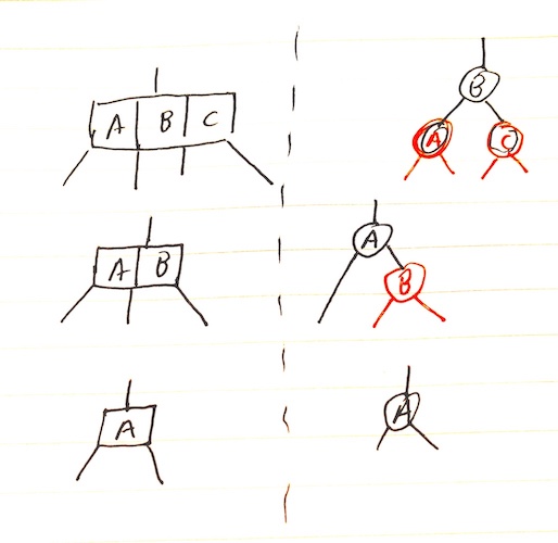
Red black trees are isomorphic to 2-3-4 trees, but has the advantage that it is easier to code:

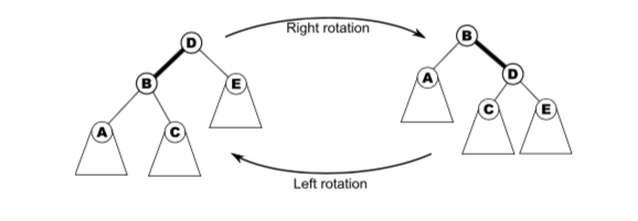
Operations that don’t modify the tree structure are the same as for BSTs. But in order to preserve the RBT invariants, other operations require rotations.

In the diagram above, D has been rotated to the right, then B has been rotated to the left. These rotations apply to non-root nodes as well.

To rotate a parent x right given its left child y:

if y != null:
    x.l = y.r
    y.r = x
    x = y

Likewise, a left-rotation:

if y != null:
    x.r = y.l
    y.l = x
    x = y

RBT Insertion

• Let p denote the parent, g the grandparent, u the uncle, and n the new node to be inserted.
• If p is black, we can just insert a red child directly.
• If p is red, we will insert a red n then clean up the tree. In this case, g must be black (because the tree cannot have two red nodes in a row).

Case 1 – red uncle

• Easy: flip colour of p, u, g.
• If g is a root, just recolour it black and finish.
• If g has a red parent, we have moved the problem up two levels.

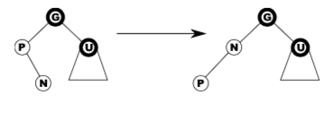
Case 2 – black uncle, bent

Left-rotate n and we are now in case 3.

Case 3 – black uncle, straight

• Swap colours of p and g, then right-rotate g.

B-tree

• B-trees are a generalisation of BSTs with a high branching factor, with the idea that children may actually be stored on a separate disc.
• Each node of a B-tree has a lower and upper bound on the number of keys it may contain (except the root has no lower bound).
• A B-tree is parameterised by a minimum degreee t such that each node will have between t and 2t pointers. A 2-3-4 tree is thus a B-tree of degree 2.
• Insertion is generalised from 2-3-4 trees: on the way down, whenever you find a full node, split it into two and move the median key up one level. Insertion can only happen in the bottom level.

B-tree deletion

• We can only delete a key from the bottom otherwise its children lose their separator. Hence we start by replacing the key with its successor like with BSTs.
• But we must prepare the tree first, because deleting might violate the minimum fullness requirement.
• Hence if deletion would cause the node to become too small, we refill a node, redistributing some keys from its siblings if they can afford to lose some, or merging.
• Merging siblings makes the parent lose a key, so we might have to recursively refill the parent.

def delete(k):
    if k is in bottom node B:
        if B cannot lose key:
            refill(B)
        delete k from B
    else:
        swap(k, successor(k))
        # now k is in a bottom node
        delete(k)

def refill(B):
    """
    PRECONDITION: B has t-1 keys
    POSTCONDITION: B has more than t-1 keys
    """
    if either sibling can lose keys:
        redistribute keys to B
    else:
        # B and all siblings have t-1 keys
        merge B with a sibling
        if B.parent has fewer than t-1 keys:
            refill(B.parent)

Hash-tables

• A hash-table is a data structure that may be used to implement the dictionary ADT.
• Keys are mapped to an integer between 0 and $m-1$ with some hash function $h(k)$, and can then be stored at that index in an array of size m.
• If two keys map to the same location, there is a hash collision. This can be resolved by chaining or open-addressing
• Chaining is a simple solution:
  • Each array location points to a linked list.
  • With a good hash function, keys will be evenly distributed in the array.
  • Worst case is $O(n)$ if all items hash to one bucket.

Open addressing

• $h(k)$ is the first preference for where to store a given key. If it is already full, we use some rule to probe the hash table for another position.
• We then follow this succession rule every time we query an item, checking for key equality.
• When an item is deleted, it should be marked as deleted rather than just removed – otherwise it interferes with the probing.

• If insertion causes the occupancy to increase beyond a certain threshold, the size of the hash table should be increased (like with dynamic arrays).

• Linear probing simply finds the next available memory cell and inserts it there.
  • return $h(k) + j \mod m$, where j is the number of attempts
  • leads to primary clustering, in which failed attempts hit the same bucket and overflow to the same buckets, resulting in long runs of occupied buckets
• Quadratic probing is an improvement that increases the space between guesses:
  • return $(h(k) + cj + dj^2) \mod m$
  • doesn’t suffer from primary clustering, but suffers from secondary clustering in which two keys that hash to the same value lead to the same probing sequence.
• Double hashing suffers from neither primary nor secondary clustering:
  • return $h_1(k) + j h_2(k) \mod m$ using different hash functions.
  • thus keys that hash to the same value will have different probing sequences
  • best open-addressing scheme in terms of collision reduction but has overhead of extra hash

Binary heap

• A heap is an almost full binary tree which satisfies the heap property, where each node has a value at least as large as those of its children. Thus the root node is the maximum element.
• The height of a binary heap is $\left \lfloor \lg n \right \rfloor$.
• Isomorphic to an array where a[k] >= a[2k+1] and a[k] >= a[2k+2].
• Min-heaps can be used to implement the priority queue ADT, allowing for easy access of the highest priority item.
• All operations are bounded by $O(\lg n)$ except for merging, which can only be done in $O(n)$ by concatenating the two arrays and heapifying.

Binomial heap

• One problem with binary heaps is that they have an $O(n_1 + n_2)$ cost to merge (concatenate arrays then heapify).
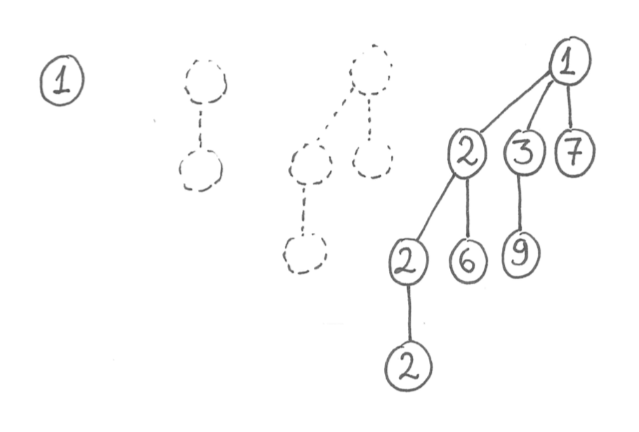
• A binomial tree of order 0 is a single node (height 0).
• A binomial tree of order k is obtained by combining two binomial trees of order $k-1$.
  • contains $2^k$ nodes
  • height is always equal to order

• A binomial heap is a forest of binomial trees, at most one of each order.
  • if a heap contains n nodes, it contains $O(\lg n)$ binomial trees, the largest of which has order $O(\lg n)$.
  • can be thought of as a binary number
• first is $O(\lg n)$ because we have to scan through the root of each binomial tree in the heap.
• Merging is very similar to binary addition, and is thus $O(\lg (n_1 + n_2))$.
• popmin requires $O(\lg n)$ to find the minimum. The children of this minimum are another binomial heap, so after deleting the minimum we can merge it with the rest in $O(\lg n)$.
• push can be viewed as merging a new binomial heap which only contains a tree of order 0. It is $O(1)$ amortised because most operations don’t touch many trees, but $O(\lg n)$ worst case.

Fibonacci heap

• Designed to make Dijkstra’s algorithm more practical by offering amortised $O(1)$ push and decreasekey.
• Idea is to be lazy for these operations, only cleaning up when popmin is called.
• Uses a list of heaps (pointers to roots), as well as a pointer to minroot.
• push creates a new heap with one node, adds it to the list of heaps, and updates minroot if necessary.
• popmin requires cleanup:
  • delete the minroot node, then promote its children to be roots
  • while there are two roots with the same degree, merge them.
  • update minroot

def push(k, v):
    h = new heap(k, v) # only one node
    add h to rootlist
    update minroot if k < minroot.key
    
def popmin():
    min = copy(minroot)
    for child in minroot.children:
        clear child mark
        add child to rootlist
    delete minroot
    cleanup()
    minroot = minimum of rootlist
    return min
    
def cleanup():
    """
    To cleanup, we use an auxiliary array where the index corresponds
    to the degree. If there is already a tree in an index, merge.
    """
    root_array = [None, None, ...]
    for tree t in roots:
        x = t
        while root_array[x.degree] is not None:
            u = root_array[x.degree]
            root_array[x.degree] = None
            x = merge(x, u)
        root_array[x.degree] = x
    return [root for root in root_array if root is not None]

• decreasekey is slightly more complicated:
  • instead of just dumping heap violations into the list, we may also need to dump its parent. Otherwise the minroot heap might be wide and shallow, leading to slow popmin
  • if you lose one child, you get marked as a loser node
  • if you lose two children, you get dumped into the root list and the mark is removed.

def decreasekey(v, new_key):
    let n be the node containing v
    n.key = new_key
    if n violates heap condition:
        repeat:
            p = n.parent
            remove n from p.children
            insert n into rootlist, updaing minroot
            n.loser = False
            n = p
        until p.loser == False
        
        if p not in rootlist:
            p.loser = True 

Analysis using potentials

• We need $\Phi$ to increase for push and decreasekey to build up for the expensive popmin, which does all the cleanup. Each push and decreasekey adds a root, while popmin removes the loser mark. Thus:

• Every push has $\Delta \Phi = 1$, so the cost is $O(1)$ amortised.
• For decreasekey, the cost depends on whether the parents are losers etc, but the total amortised cost is still $O(1)$.
• The cost of popmin will depend on $d_{max}$, the upper bound on the degree of any node in the heap.
  • promoting the children of minroot has true cost $O(d_{max})$, and the same amortised cost.
  • cleanup is $O(d_{max})$ as well.

Relationship to Fibonacci numbers

• As a consequence of the grandchild rule, if a node in a Fibonacci heap has d children, then that the subtree rooted at that node has more than $\geq F_{d+2}$, where F is a Fibonacci number.
• Consider a node x in the Fibonacci heap, with children $y_1, y_2, \ldots, y_d$ in the order which they became children of x.
• When x acquired $y_2$, it already had $y_1$, so $y_2$ must have had $\geq 1$ child for it to be merged. Likewise, $y_3$ must have had $\geq 2$ children, $y_d$ must have had $\geq d -1$ children.
• But decreasekey could have caused them to lose at most one child.
• The total number of nodes is then bounded by:

• Where $N_0 \geq 0$, corresponding to either $y_1$ or $y_2$.
• Thus by definition of the Fibonacci numbers: