Foundations of Computer Science
Contents
- Basic syntax
- Expressions and complexity
- Lists
- Sorting
- Datatypes
- Binary trees
- Search strategies
- Functions as values
- Lazy lists
- Polynomial arithmetic
- Procedural programming
Basic syntax
- Computing is largely about abstraction: what services should be provided at different levels and how should these interface?
- The goal of programming is to describe computation mechanically, allowing for correct, efficient and maintainable code.
- ML abstracts away the underlying hardware (and memory management), and is similar to mathematics.
This is a value declaration with pi as the identifier.
val pi = 3.1415;
If we compute an expression, ML actually declares an identifier it and sets it to the value of the computed expression. We can also perform a simultaneous declaration using val a=1 and b=2 (which can also be used to swap names).
Functions are also values, just with a special declaration syntax. This invites the use of recursion:
fun npower (x, n): real =
    if n = 0
    then 1.0
    else x * npower (x, n-1);
> val npower = fn : real * int -> real
fun gcd (m,n) =
    if m = 0 then n else gcd (n mod m, m);
All ML functions only operate on one argument. The type signature real * int specifies that this argument is a (real, int) tuple.
Operators are overloaded between different types: e.g. multiplication is a different operator for reals and integers but in both cases it uses *. Some operators are different, for example / is not defined for integers (div must be used instead). All the operators (infix or not) are treated as functions, and therefore as values.
~;
> val it = fn: int -> int
Infix operators can be defined:
infix ||;
fun x || y = x*x + y*y;
Although ML usually infers types, in ambiguous cases it is best to provide a type annotation as follows:
fun square (x: real) = x * x
In ML, = is both used for assignment and equality. In general we should only do equality testing if the arguments are of the same type. Inequality is tested for using <>.
Conditional expressions take the form:
if p then E1 else E2
p is a predicate - a boolean expression that determines which of E1 or E2 is evaluated. The boolean operators are not, andalso, orelse. The latter two are not functions because they only evaluate the second expression if needed. They are just shorthand, e.g. p andalso q $\equiv$ if p then q else false.
e.g. efficiently raising a number to a power:
fun power (x: real, n) =
    if n = 1 then x
    else
        if (n mod 2 = 0) then power(x*x, n div 2)
        else x * power(x*x, n div 2);
ML determines the type of an expression without computing the expression
Expressions and complexity
Expression evaluation is a model for computation in which an expression $E_i$ reduces to an expression $E_{i+1}$ until this process concludes with value v. We write $E_i \implies E_{i+1}$ rather than $E_i = E_{i+1}$ because computation is typically one-way. Functional programming deals with expressions and resulting values rather than states.
ML’s evaluation rule is call-by-value (or strict evaluation), rather than call-by-need (lazy) evaluation. To compute the value of $f(E)$, it first computes the value of $E$.
It is possible to have iteration in a functional paradigm using tail recursion. This is done by adding an accumulator argument which keeps track of some total. Compared to the recursive approach, iterative solutions tend to require much less space. However, the additional parameters can sometimes reduce clarity.
fun iterateFactorial (n, total) =
    if n = 0 then total else iterateFactorial(n - 1, n * total);
We can attempt to analyse the quality of algorithms by considering their time and space complexity as a function of input size n. This is usually considered asymptotically using big O notation. We say that:
\[f(n) \subseteq O(g(n)) \qquad \text{if} \qquad |f(n)| \leq c | g(n)|\]Similarly, we can define $\Omega(g(n))$ if g is the lower bound and $\Theta(g(n))$ if g is both the lower and upper bound.
\[O(1) \subseteq O(\log n) \subseteq O(n) \subseteq O(n \log n) \subseteq O(n^2) \subseteq O(a^n)\]Time complexity must be greater than or equal to space complexity, because the space must be traversed.
Tail recursive algorithms often have constant space complexity because they only need to store one value.
We can find the big O complexity by finding a recurrence relation on the cost function $T(n)$, assuming a base case of $T(0) = 1$ or $T(1) = 1$.
| Recurrence | Big O complexity |
|---|---|
| $T(n+1) = T(n) + 1$ | $O(n)$ |
| $T(n+1) = T(n) + n$ | $O(n^2)$ |
| $T(n+1) = 2T(n/2) + 1$ | $O(\log n)$ |
| $T(n+1) = 2T(n/2) + n$ | $O(n \log n)$ |
Lists
A list is a finite ordered series of elements of the same type. It is built from two primitives:
[](ornil) is the empty list. This is polymorphic and has type'a list.::is the cons operator, such thatx::lis the list with headxand taill.- Cons is an $O(1)$ operation because under the hood ML is using linked lists.
Strings
Strings are not treated purely as lists of characters. There are special methods for strings:
explodeconverts a string into a list of charsimplodedoes the oppositesizefinds the number of chars in a stringa ^ bfor concatenation.
List functions
There are two useful built-in functions:
- The infix append operator
@. The operationxs @ ysis $O(xs)$: in general it is much better to use cons directly. - The function
revto reverse a list in $O(n)$.
We can define functions with separate clauses in order to pattern-match.
fun nlength [] = 0
  | nlength (x::xs) = 1 + nlength xs;
For list functions, sometimes using cons instead of append leaves the result the wrong way round. The cost of rev should be considered.
We can define functions to take or drop the first k elements as follows:
fun take ([], _) = []
  | take (x::xs, k) =
        if (k > 0) then x::take(xs, k-1)
        else [];

fun drop ([], _) = []
  | drop (x::xs, k) =
        if (k > 0) then drop(xs, k-1)
        else (x::xs);
Although these functions have the same complexity, drop will be faster (i.e smaller constant factor) because it is discarding elements.
Searching
To find an item in a list, we can loop through items in a linear search with $O(n)$ complexity. If the list is indexed (as in a hash table), lookup is $O(1)$.
fun member (x, []) = false
  | member (x, y::ys) =
        (x=y) orelse member (x, ys);
> val member = fn: ''a * ''a list -> bool
In the type signature, ''a means that the function only accepts equality types. This includes most types except:
- reals (because of floating point issues)
- functions, because there is no way of knowing a priori whether the output would be the same for all possible input.
- abstract types
Zipping and Unzipping
We desire:
zip: ('a list * 'b list) -> ('a * 'b) list
unzip: ('a * 'b) list -> ('a list * 'b list)
Because patterns are tested in order, we can write a zip function as follows:
fun zip (x::xs, y::ys) = (x, y) :: zip(xs, ys)
  | zip _              = []
If there is a case where one of the lists is empty, the first pattern will not match so the second will just produce an empty list.
The unzip function is best written with a local declaration:
fun unzip [] = ([], [])
  | unzip ((x,y)::pairs) =
        let val (xs, ys) = unzip pairs
        in (x::xs, y::ys)
        end;
It could be more obviously written with accumulator arguments, but we will then have to reverse it.
Making change
The simplest greedy algorithm is straightforward to implement, noting that:
- Change for zero consists of no comparisons
- Otherwise we try the largest available and reduce the outstanding coin. Discard if the coin is too large.
fun change (till, 0) = []
  | change (c::till, amt) =
        if amt<c then change(till, amt)
        else c::change(c::till, amt-c);
However, this greedy algorithm can fail in simple cases. We can define an exhaustive iterative solution as follows, where chg is the current solution and chgs is the list of solutions:
fun change (till, 0, chg, chgs) = (chg::chgs)
  | change ([], _, chg, chgs) = chgs
  | change (c::till, amt, chg, chgs) =
        let
            val otherSol = change(till, amt, chg, chgs)
        in
            if amt<0 then chgs
            else change(c::till, amt-c, c::chg, otherSol)
        end;
- In the base case, we cons the current
chgto a list of all possiblechgsand return it. - At any point, if
amtis zero, we stop and returnchgs. - Otherwise, we deduct the coin at the top of the till from
amtand continue (same as in greedy). At the same time we recursively explore other possibilities (e.g. ignore the biggest coin even if we can use it).
Defining a set
We can emulate functioning of a set using lists. We want:
- Membership testing
- Adding an item
- Converting a list to a set
- Union
- Intersection
fun mem (x, []) = false
  | mem (x, y::ys) = (x=y) orelse mem (x, ys);

fun addmem (x, l) = if mem (x, l) then l else x::l;

fun setof [] = []
  | setof (x::xs) = addmem(x, setof xs);

fun union ([], l) = l
  | union (x::xs, l) = union(xs, addmem(x, l));

fun intersect ([], l) = []
  | intersect (x::xs, l) =
        if (x mem l) then x::intersect(xs,l)
        else intersect(xs, l);
Sorting
Sorting is important because searching a sorted collection only requires $O(\log n)$ time (via a binary search) compared to $O(n)$ time for a linear search.
Efficiency of sorting algorithms is analysed by considering the number of comparisons that must be made. The optimal complexity of a comparison-based algorithm must be $O(n \log n)$, which can be seen by noting that in the best case each comparison eliminates half of the permutations.
\[2^{C(n)} \geq n! \implies C(n) \geq \log_2(n!) \approx n \log n - 1.44n\]Insertion sort
Works by recursively inserting elements into sorted lists.
fun ins(x, []) = [x]
  | ins(x, y::ys) =
        if (x <= y) then x::y::ys
                    else y::ins(x, ys);

fun insort [] = []
  | insort (x::xs) = ins(x, insort xs);
insinserts an element into a sorted list, and requires $n/2$ comparisons on average (worst case n).insortcallsinson average n times, so the overall algorithm is $O(n^2)$.
Quicksort
Quicksort is a divide and conquer algorithm:
- Choose a pivot element a
- Partition the list into one with elements greater than a and the other with elements ≤ a (this is an $O(n)$ operation).
- Sort sublists, then append together.
fun quick [] = []
  | quick [x] = [x]
  | quick (pivot::xs) =
      let fun part (l, r, []) = (quick l) @ (pivot::quick r)
            | part (l, r, y::ys) =
                    if y <= pivot
                    then part (y::l, r, ys)
                    else part (l, y::r, ys)
      in part ([], [], xs) end;
In the average case, quicksort is $O(n \log n)$. If the pivot divides the input into two equal parts at every step, we have
\[T(n) = n + 2T(n/2) = O(n \log n)\]In the worst case, all but one of the items end up in one partition so we have:
\[T(n+1) = n + T(n) = O(n^2)\]In both cases, the $n$ comes from the partition (and the append in ML). An iterative version would have the same complexity but would have $n$ rather than $2n$ since it doesn’t append.
Mergesort
The merge function merges two sorted lists (but doesn’t work well for arrays), requiring at most $m+n$ comparisons.
fun merge ([], ys) = ys
  | merge (xs, []) = xs
  | merge (x::xs, y::ys) =
        if x <= y then x :: merge(xs, y::ys)
        else y :: merge(x::xs, ys);
Mergesort splits a list in two, recursively sorts sublists, then combines them using merge.
fun mergesort [] = []
  | mergesort [x] = [x]
  | mergesort xs =
      let val k = (length xs) div 2
      in merge (mergesort (take(xs, k)), mergesort(drop(xs, k)))
      end;
Because take and drop divide the list into two equal parts, the complexity is always $O(n \log n)$ because:
In practice, quicksort is slightly faster (except for the worst case complexity).
Datatypes
ML allows us to declare new types using the datatype declaration. The identifiers of a new type are called constructors:
datatype vehicle = Bike
                |  Car
                |  Lorry
These types are treated as if they were built-in, so we can write functions on datatypes with pattern matching. The previous example is just an enumeration type. We can associate data with each constructor as follows:
datatype vehicle = Bike of int (*n wheels*)
                |  Car of bool (*diesel or not*)
Exceptions
Raising an exception abandons the current computation; handling the exception attempts an alternative.
(* exception Failure *)
exception Failure;
exception HttpError of int;

raise Failure;
raise (HttpError 404);
Exception names are constructors of the builtin datatype exn, meaning that exception handlers can pattern match.
E handle Failure => E1
    | (HttpError 404) => E2;
Using exceptions we can write a backtracking algorithm to make change:
fun change (till, 0) = []
  | change ([], amt) = raise ChangeError
  | change (c::till, amt) =
        if amt < 0 then raise ChangeError
        else (c :: change(c::till, amt - c))
        handle ChangeError => change(till, amt);
If a particular choice of coin makes it impossible to find change in the next recursive call, the handler undoes the most recent choice. If making change is impossible, the second pattern will eventually match and the ChangeError will be raise with no handler.
An alternative to exceptions is to declare an option datatype, but this requires constant checking for NONE
datatype 'a option = NONE | SOME of 'a;
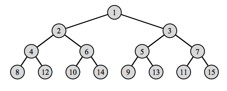
Binary trees
The binary tree is built on a recursive datatype, wherein each node is either empty (i.e nil), or two subtrees.
datatype 'a tree = Lf
                | Br of 'a * 'a tree * 'a tree;
Declaring a tree:
val tr = Br(1, Br(2, Br(4, Lf, Lf), Br(5, Lf, Lf)), Br(3, Lf, Lf));
Simple tree functions:
fun count Lf = 0
  | count (Br(v, t1, t2)) = 1 + count(t1) + count(t2);

fun depth Lf = 0
  | depth (Br(v, t1, t2)) = 1 + Int.max(depth t1, depth t2);
Dictionaries and binary search trees
A dictionary is an abstract type with the following components
- lookup
- update (insert)
- delete
- empty (a null dictionary)
- missing exception
Using a list of (k,v) pairs entails $O(n)$ lookup. A binary search tree can be used instead as long as the keys have a total ordering. Each branch of the tree carries a (k,v) pair. The left subtree contains smaller or equal keys; the right subtree contains greater keys. For a balanced tree, update and lookup are both $O(\log n)$.
exception Missing;

fun lookup (Br ((k, v), t1, t2), a) =
    if a < k then lookup (t1, a)
    else if a > k then lookup (t2, a)
    else v;
  | lookup (Lf, a) = raise Missing;

fun update (Lf, k, v) = Br((k,v), Lf, Lf)
  | update (Br((a,b), t1, t2), k, v) =
        if k < a then Br((a,b), update (t1, k, v), t2)
        else if k > a then Br((a,b), t1, update (t2, k, v))
        else (*overwrite*) Br((a,v), t1, t2);
This update function overwrites if the keys are equal. Unchanged parts of the tree are shared (under the hood), so this is efficient.
Traversing trees
Trees can be traversed in three ways:
- preorder - label, left subtree, right subtree
- inorder – left subtree, label, right subtree
- postorder - left subtree, right subtree, label.
- Breadth-first (discussed later).
These can be very clearly implemented using @, but this has quadratic complexity.
fun inorder Lf = []
  | inorder (Br(v, t1, t2)) = inorder t1 @ [v] @ inorder t2;
Instead, the functions should be defined using an accumulator.
fun preorder (Lf, vs) = vs
  | preorder (Br(v, t1, t2), vs) =
            v :: preorder (t1, preorder (t2, vs));

fun inorder (Lf, vs) = vs
  | inorder (Br(v, t1, t2), vs) =
            inorder (t1, v::inorder (t2, vs));

fun postorder (Lf, vs) = vs
  | postorder (Br(v, t1, t2), vs) =
            postorder (t1, postorder (t2, v::vs))
Functional arrays
A functional array is a finite map from integers to data. Updating the array is not an imperative command, rather it is a function that returns the updated array.
A functional array can be represented as a binary tree. The position of subscript k is determined by starting at the root and repeatedly (integer) dividing k by 2. At each stage, if the remainder is zero, move it to the left subtree. Otherwise right.
exception Subscript;

fun sub (Lf, _) = raise Subscript;
  | sub (Br(v, t1, t2), k) =
        if k = 1 then v
        else if k mod 2 = 0 then sub (t1, k div 2)
        else sub (t2, k div 2);

fun update (Lf, k, w) =
        if k = 1 then Br(w, Lf, Lf)
  | update (Br(v, t1, t2), k, w) =
        if k = 1 then Br(w, t1, t2)
        else if k mod 2 = 0
            then Br(v, update(t1, k div 2, w), t2)
        else Br(v, t1, update(t2, k div 2, w));

fun delete (Br(v, Lf, Lf)) = Lf
  | delete (Br(v, Br(w, t2, t3), t1)) =
                    Br(w, t1, delete(Br(w,t2,t3)));
Search strategies
A stack is a data structure that lets you add, discard, or return to/from the top only. It can be easily implemented with ML lists. We can use a stack to store the trees in a depth-first search.
Queues and breadth-first search
In order to search a tree breadth-first, we keep a list of trees to visit, and do not traverse those until we have visited the nodes at the current depth. A naive list implementation would be very inefficient because we must append the trees to the back.
A queue is a FIFO data structure with the following functions:
enqadds an element at the end.qhdreturns the first elementdeqdiscards the element at the head
We can represent a queue as a pair of lists: the front half of the queue is stored in the first list, and the second half is stored in reverse order in the second list.
datatype 'a queue = Q of 'a list * 'a list;

fun norm (Q([], tls)) = Q(rev tls, [])
  | norm q = q;

fun enq (Q(hds, tls), x) = norm(Q(hds, x::tls));
fun deq (Q(x::hds, tls)) = norm(Q(hds, tls));
fun qhd (Q(x::_, _)) = x;
enq will then always be constant time. deq will be $O(1)$ except when the front list is empty, in which case we must normalise the queue (reversal is $O(n)$). Thus on average, for n enqueues and dequeues, there will be $O(n)$ operations, so the amortised complexity is $O(1)$. But because this complexity is not evenly distributed, this data structure may not be suitable for real-time programming.
Using a queue, the breadth-first traversal is:
fun breadth q =
    if qnull q then [] else
    case qhd q of
        Lf => breadth (deq q)
      | Br(v, t1, t2) => breadth (enq(enq(deq q, t1), t2));
Depth-first iterative deepening
The main problem with BFS is that it has exponential space complexity: it keeps track of $O(b^d)$ nodes (for a binary tree, $2^d -1$ nodes).
Iterative deepening searches the tree repeatedly, each time bounded by a finite depth. The time complexity of this is only $b/(b-1)$ greater than BFS, because of the exponential growth. But the space requirement is that of a DFS, i.e $O(d)$.
Functions as values
ML allows for functionals (higher-order functions) which operate on other functions (because functions are just values). We can define these as anonymous lambda functions:
fn x => x**x;
> val it = fn : int -> int
In ML, all functions have exactly one argument. Previously we have been passing tuples, but an alternative is to use currying. A curried function returns another function as its result. They allow for partial application.
ML has a builtin map functional, which could be defined as follows:
fun map f [] = []
  | map f (x::xs) = (f x) :: map f xs;

 > val it = fn: ('a -> 'b) -> 'a list -> 'b list
Note that the -> symbol associates to the right, so we actually have: ('a -> 'b) -> ('a list -> 'b list), i.e map takes in some polymorphic function and returns a function that converts an input list into the mapped list.
We can apply map to matrix transposes and products:
fun hd (x::_) = x;
fun tl (_::xs) = xs;

fun transp ([]::_) = []
  | transp rows = (map hd rows) :: (transp (map tl rows));

fun dot [] [] = 0
  | dot (x::xs) (y::ys) = x*y + (dot xs ys);

fun matprod (Arows, Brows) =
    let val cols = transp Brows
    in map (fn row => map (dot row) cols) Arows
    end;
dot row is partially applied to all of the columns in B.
List functionals for predicates
These functionals transform a predicate into a predicate over lists.
fun exists p [] = false
  | exists p (x::xs) = (p x) orelse exists p xs;

fun filter p [] = []
  | filter p (x::xs) =
        if p x then x :: filter p xs
        else filter p xs;

fun all p [] = true
  | all p (x::xs) = (p x) andalso all p xs;
These can be used to simplify many set operations:
fun mem (x, l) = exists (fn y => y=x) l;

fun inter (xs, ys) = filter (fn x => mem (x, ys)) xs;
Lazy lists
Sequential programs accept an input problem, processes it, then terminates. Reactive programs interact with the environment, and are event-triggered, e.g. in the following pipeline
producer -> filter -> ... -> filter -> consumer
The consumer requests and consumes results: nothing is computed otherwise. A simple way to model this in ML is with lazy lists (a.k.a sequences):
- allow for delayed evaluation
- can be unbounded
- not quite the same as lazy evaluation.
We can delay evaluation by using the empty tuple () (of type unit).
fn f () => E
Note that E is not evaluated until f is called. We can use this to define a sequence of the form Cons(x, xf), where x is the head and xf is a delayed function to compute the tail.
datatype 'a seq = Nil
                | Cons of 'a * (unit -> 'a seq);

fun head (Cons(x, _)) = x;
fun tail (Cons(_, xf)) = xf();

fun from k = Cons(k, fn() => from(k+1));

fun get(0, xq) = []
    | get (n, Nil) = []
    | get (n, Cons(x,xf)) = x :: get (n-1, xf());
Rather than appending sequences (which fails if one is infinite), it may be better to interleave:
fun interleave (Nil, yq) = yq
  | interleave (Cons(x, xf), yq) =
                Cons(x, fn() => interleave(yq, xf()));
We can define functionals with boolean predicates, which can be useful to produce a list of a certain type:
fun filterq p Nil = Nil
  | filterq p (Cons(x, xf)) =
        if (p x) then Cons(x, fn() => filterq p (xf()))
        else filterq p (xf());

fun iterates f x = Cons(x, fn() => iterates f (f x));
Polynomial arithmetic
Programming involves finding data representations for abstract concepts. For example, we may try to implement finite sets:
- We will represent the abstract concept with concrete objects - repetition-free lists.
- The abstract object will be represented by at least one concrete object e.g.
{3,4,5} -> [3,4,5]. - There may be concrete objects that do not represent an abstract object, e.g.
[3,3,5]. - Operations on the abstract data must preserve the representation.
We will represent the polynomial $a_n x^n + \cdots + a_1x + a_0$ as a sparse (int*real)list, with real (nonzero) coefficients and decreasing exponents.
e.g. $~x^{500} - 2x + 3 \rightarrow$ [(500, 1.0), (1, ~2.0), (0, 3.0)].
The polynomial sum is easy to implement but we must be careful to check all cases to preserve the representation.
fun polysum [] us = us :(int*real) list
  | polysum ts [] = ts
  | polysum ((m,a)::ts) ((n,b)::us) =
        if m > n then (m,a):: polysum ts ((n,b)::us)
        else if m < n
            then (n, b) :: polysum us ((m,a)::ts)
        else if a+b = 0.0 then polysum ts us
             else (m, a+b) :: polysum ts us;
In order to multiply polynomials, we can map a pairwise product over both polynomials
fun termprod (m,a) (n,b) = (m+n, a*b);

fun polyprod [] us = []
  | polyprod ((m,a)::ts) us =
        polysum (map (termprod (m,a)) us)
                (polyprod ts us);
This function is inefficient because polysum will have to merge lists with lengths that differ greatly. We can improve it in the style of mergesort:
fun polyprod [] us = []
  | polyprod [(m,a)] us = map (termprod (m,a)) us
  | polyprod ((m,a)::ts) us =
        let val k = length ts div 2
        in polysum ((polyprod (take(ts, k)) us))
                   ((polyprod (drop(ts, k)) us))
        end;
Polynomial division can be done using the standard algorithm to return a (quotient, remainder) tuple.
- If the divisor is empty, there is no remainder so return the quotient (must be reversed because we accumulated with cons).
- If the degree of the numerator is smaller than that of the denominator, return the numerator as the remainder.
- Otherwise divide out the leading power, multiply out, then subtract.
fun polydivide ts ((n,b)::us) =
  let fun quo []         qs = (rev qs, [])
       |  quo ((m,a)::ts) qs =
            if m<n then (rev qs, (m,a)::ts)
            else
            quo (polysum ts
                        (map termprod(m-n, ~a/b) us))
                ((m-n, a/b) :: qs)
 in quo ts [] end;
Procedural programming
Procedural programming involves transforming state through commands or statements. Though functional programming abstracts away the state, in reality it still must deal with storage.
ML models memory as mutable cells, and provides the following primitives for references:
'a refis the type of a reference to an $\alpha$ type value.val P = ref Ecreates an $\alpha$ type reference – i.erefis also function that returns an'a ref.!Preturns the current contents of reference P (dereferencing).P := Eupdates the contents of P to the value of E
Values in ML are immutable – only memory cells support reassignment. In the below example, ps doesn’t change, only the contents of the reference at its head do.
val ps = [ref 77, ref 6];
hd ps := 3;
ML uses aliasing - if you assign a new reference to equal an old one, updating either will update both. In order to make references ‘private’, we can design “factory methods” that return functions with their own references.
Commands and control flow
A command is an expression that affects state, normally returning unit. Multiple commands can be executed using $C_1; C_2; \ldots; C_n$. This evaluates each expression but only returns $C_n$.
This can be used in while loops, which evaluate some statements until the predicate is false.
while B do (C1; C2; C3);
Because of the way commands are evaluated, we can make a do-while loop as follows:
while (C1; B) do (C2; C3);
Arrays
ML arrays can be thought of as references that contain several elements. The array primitives are:
'a Array.array- an array that contains $\alpha$ type valuesArray.tabulate(n, f)creates an n-element array whereA[i]holds $f(i)$Array.sub(A,i)returns the contents ofA[i]Array.update(A,i,E)updatesA[i]to the value of E.
These arrays are safer than C arrays because they are still abstracted (i.e you can’t edit the machine’s memory). However, they are less flexible (e.g. for 2D arrays).
Example: mutable linked lists
We can implement mutable linked lists using a custom recursive datatype, representing it as a head and a reference to the rest of the list.
datatype 'a mlist = Nil
                  | Cons of 'a * ('a mlist ref);

fun mlistOf [] = Nil;
  | mlistOf (x::l) = Cons(x, ref (mlistOf l));

fun extend (mlp, x) =
  let val last = ref Nil
  in mlp := Cons(x, last);
     last;
  end;
The extend function accepts a reference to a list and a new value. It is important that it returns last: this is needed so that we can add values via extend (it, newVal).