Probability matching and Kelly betting

In this post, we discuss a cognitive bias called probability matching, explaining how it is rational from a population perspective. We then make an analogy to the Kelly criterion, a betting strategy that finds widespread use in both gambling and finance.

Probability matching

I probably don’t need to tell you that humans aren’t perfectly rational utility-maximisers – thanks to the work of heavyweights like Kahneman and Tversky, the existence of cognitive biases is widely appreciated (in theory, if not in practice). Books like Thinking, Fast and Slow catalogue some of these biases.

Today I want to discuss one in particular: probability matching.

Consider a weighted coin that comes up heads 75% of the time. I am going to flip this coin many times; before each flip, you can guess whether it will be heads or tails. Your goal is to maximise the number of correct guesses. What is your strategy?

The optimal strategy is to guess H every time, which should mean that 75% of your guesses are correct.

But animals (humans included) seldom choose this strategy¹. Rather, they guess H about 75% of the time, matching their guessing frequency to the probability – probability matching.

Let the coin have a known $P(\text{heads}) \equiv p > 0.5$ and consider a strategy in which we choose heads with frequency f. Assume that we receive a payout of +1 for a correct guess and -1 for an incorrect guess. The expected value per coin toss is $EV = 1 - 2(f+p-2fp)$.

In the “optimal” case $f=1$ (i.e we always guess H provided $P(\text{heads}) > 0.5$), we gets $EV = 2p-1$. Probability matching, in which we set $f=p$, yields $(2p-1)^2$.

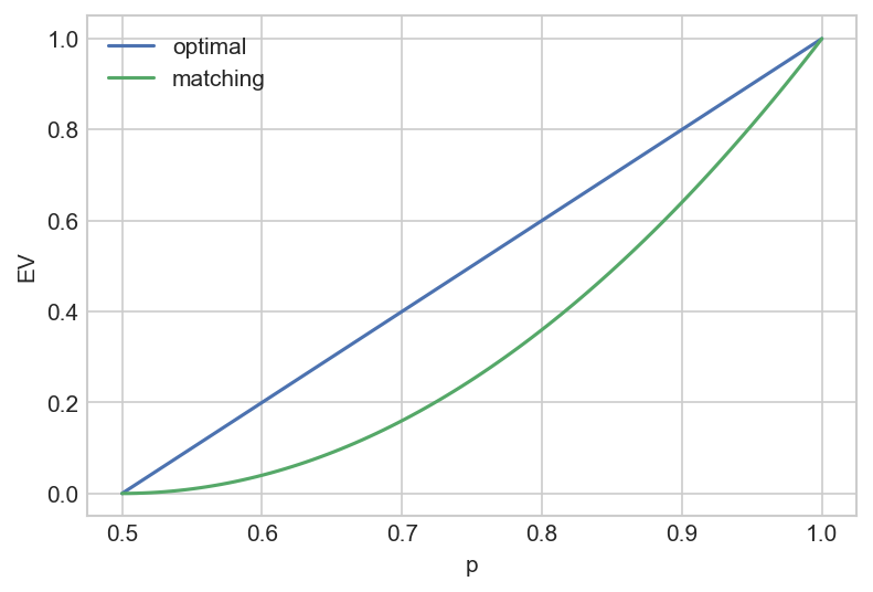
Hence probability matching is a cognitive bias to the extent that it is a mathematically suboptimal strategy that results in a lower expected value.

The rationality of probability matching

In their 2011 paper The Origin of Behaviour, Brennan and Lo make the wonderful insight that while probability matching is suboptimal from an individual level, it may be rational from a population level.

To motivate this, we’ll move from coin flips to a more ecological example.

You are an arctic fox trying to decide whether or not to change your coat from brown to white for the winter. If you have the wrong coat colour, i.e you turn white but it doesn’t snow, or you stay brown and it does snow, you get eaten by predators (sorry, I don’t make the rules). If you have the correct coat colour you survive and reproduce. The probability of no snow in winter is 75%. What is your strategy?

The best strategy for an individual fox is to always stay brown as long as $P(\text{no snow}) > 0.5$.

But consider the population perspective: if every fox stayed brown, then it would only take one winter with snow for the entire fox population to be wiped out. So the optimal strategy at a population level cannot be for every fox to stay brown, even though that is optimal for an individual!

Hopefully, this example illustrates intuitively why probability matching is a plausible strategy at the population level. In the next section, we’ll explore this idea mathematically.

Optimising population growth

Let’s build out the fox model a little more. We make the following assumptions:

• The probability that it doesn’t snow in winter is $p$; the probability it does snow is $1-p$
• If a fox survives the winter (by having the right coat colour), it reproduces to make $W-1$ offspring, such that one fox becomes W foxes (W for “win”!)
• The “objective” is to maximise the population.
• Before winter, we have a population of $n_0$. A fraction $f$ of this population remains with brown coats, the other $1-f$ change to white coats.

How does the population evolve after one winter? If it doesn’t snow, the $fn_0$ brown foxes survive and reproduce to become $fn_0 \cdot W$ foxes. If the winter is snowy, the $(1-f) n_0$ white foxes reproduce to become $(1-f)n_0 \cdot W$ foxes.

To summarise, the population dynamics are:

\[n_0 \to \begin{cases} f n_0 \cdot W, & \text{no snow} \\ (1-f)n_0 \cdot W, & \text{snow} \end{cases}\]

Over T winters, we expect snow in $(1-p)T$ winters and no snow in $pT$ winters. The overall population after these T winters is then:

\[n = n_0 \cdot (fW)^{pT} \cdot ((1-f)W)^{(1-p)T}\]

The key question – what fraction $f^* $ of the population should stay brown to maximise population growth – is then just a calculus problem. We just differentiate n w.r.t f and set it to zero to find the optimal $f^*$ (though for mathematical convenience, we first take logs):

\[\begin{aligned} \ln n &= \ln n_0 + pT (\ln f + \ln W) + (1-p)T (\ln (1-f) + \ln W) \\ \frac{\partial \ln n}{\partial f} &= \frac{pT}{f} - \frac{(1-p)T}{1-f} = 0 \\ &\implies \frac p f = \frac{1-p}{1-f} \\ &\implies \frac{p}{1-p} = \frac{f}{1-f} \\ &\implies f^* = p \end{aligned}\]

So a fraction $f^* = p$ of the population should stay brown, leaving them best adapted to a winter without snow (which occurs with probability $p$) – this is exactly the probability matching rule!

Kelly betting

We now modify the model slightly.

• In a snowy winter: brown foxes die, white foxes survive but don’t reproduce.
• In a non-snowy winter: all foxes survive, but only the brown foxes reproduce (to make $W-1$ offspring as before)

This model is admittedly somewhat contrived, but is vaguely plausible:

• A snowy winter is likely a tougher environment with less food available (so even the well-adapted white foxes may not be able to reproduce easily)
• In a non-snowy winter, adaptation still matters, so the maladapted white foxes may not be desirable mates.

With this model, the population dynamics are as follows (f is again the fraction of brown foxes):

\[n_0 \to \begin{cases} n_0 (1 + fW), &\text{no snow} \\ n_0 (1-f), & \text{snow} \end{cases}\]

The population growth equation is:

\[n = n_0 (1+fW)^{pT} (1 - f)^{(1-p)T}\]

We repeat the procedure as before, choosing the $f^*$ that maximises $\ln n$.

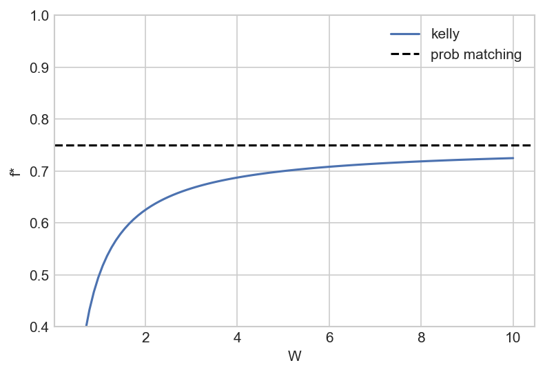
\[\begin{aligned} \ln n &= \ln n_0 + pT \ln (1+fW) + (1-p)T \ln (1-f) \\ \frac{\partial \ln n}{\partial f} &= 0 \implies \frac{pW}{1+fW} - \frac{1-p}{1-f} = 0 \\ &\implies f^* = p - \frac{(1-p)}{W} \end{aligned}\]

This is identical to Kelly betting, with the following mapping:

• n is the value of the bankroll
• f is the fraction of the bankroll that we bet
• W is the odds of the bet – the factor by which the stake grows if we win.

We can then apply the plethora of known results for the Kelly betting scheme² to understand the long-run growth trajectory of the population, the time it takes for this strategy to dominate others, etc.

However, note that in this model, probability matching is never optimal, since there is no finite W such that $f^* = p$. That said, we see behaviour similar to probability matching: for $p = 0.75$ and a reproductive factor $W = 5$, the optimal fraction is $f^* = 0.7$.

To take a step back, the reason why this ecological model is similar to Kelly betting is that in both cases the objective is to maximise the geometric growth rate – while Brennan and Lo (2011) observe the same, they don’t elucidate the link between probability matching and the Kelly frequency.

Conclusion

We’ve explored some simple models to illustrate that probability matching is rational from a population perspective. The population seeks to maximise its geometric growth rate, and therein lies the link to Kelly betting.

To clarify, probability matching is still irrational for an individual – if you are a fox you should change to a white coat if you think that there is a greater than 50% chance of a snowy winter. But your genes would be telling you otherwise!

This topic is so interesting to me because it is a first-principles derivation of a cognitive bias: it would be awesome if we could explain the full spectrum of cognitive biases at a biological level (be that neuroscience or evolution). Prospect theory is really only a phenomenological theory – it uses the S-shaped utility curve to explain several empirically observed biases, without rigorously explaining where that utility function might come from.

Lastly, a comment on an important extension. In this post, we found that the probability matching rule arises from uncertainty about the future state of the world, but we have completely neglected parameter uncertainty. In other words, we assumed that we know p, while in reality we may not know the bias of the coin, or the probability that it snows – these are parameters that must be estimated under uncertainty. In this case, answering questions about optimal strategies becomes difficult. It is an explore vs exploit tradeoff – you need to estimate p while simultaneously making decisions whose payoff depends on p! Techniques like reinforcement learning become applicable here, and ultimately these are likely to be a key part of understanding where cognitive biases come from.

References