Intuiting the gamma function, part 1

What is the factorial of a half? This series of posts builds up from middle-school algebra to the enigmatic gamma function in an attempt to answer this simple question.

When high-school students study the Binomial Theorem, a classic problem is the expansion of a binomial with a fractional power, such as $(1+x)^{1/2}$. Speaking from experience, a student’s first attempt is often to naïvely substitute values into the formula for the Binomial Theorem, leading to

\[(1+x)^{1/2} = 1 + \binom{0.5}{1}x + \binom{0.5}{2}x^2 +\ldots+x^n\]

The problem arises when trying to evaluate $\binom{n}{r}$. We could just try to use the standard formula:

\[\binom{n}{r} = \frac{n!}{r!(n-r)!}\]

but the student will soon encounter the troubling question of how to evaluate $0.5!.$ Clearly, the traditional definition of the factorial does not make any provision for non-integers.

However, it turns out that there is a natural extension of the factorial to all complex numbers excluding the nonpositive integers called the gamma function, $\Gamma (x)$, which is defined using an integral:

\[\Gamma (x) = \int_0^\infty t^{x-1}e^{-t} dt, \qquad x \in \mathbb{C}| x \not\in \left \{ \{0\} \cup \mathbb{Z}^- \right \}\]

Don’t let the t distract you: it is just a dummy variable. The gamma function is a function of x. But the question is, what on earth has this got to do with factorials? As it happens, there is a wonderful intuitive reason for the form of the gamma function, and how it relates to $x!$, which I aim to explain. Following along will require the reader to have a reasonable understanding of differentiation and integration, but I will try to assume little else.

Just a disclaimer: the maths used here isn’t going to be formally rigorous, but it will definitely be valid and hopefully intuitive.

The Factorial

For $\forall n \in \mathbb{N}$ (this means ‘for all natural numbers’), the factorial, which will henceforth be referred to as the ‘traditional factorial’, is defined by the following two conditions:

• $1! = 1$
• $n! = n(n-1)!$, the recursion condition

These two conditions alone are sufficient to calculate any integer factorials.

For example, if we needed to find $4!$, we would simply apply the recursion condition multiple times until we see a $1!$, at which point we apply condition 1:

\[4! = 4 \cdot 3! = 4 \cdot 3 \cdot 2! = 4 \cdot 3 \cdot 2 \cdot 1! = 4 \cdot 3 \cdot 2 \cdot 1 = 24\]

Now the problem is that there is no obvious way to apply these two conditions to non-integers. We could conceivably apply the recursion condition

\[2.5! = 2.5 \cdot 1.5! = 2.5 \cdot 1.5 \cdot 0.5!\]

But we are now left with the conundrum of working out $0.5!$. Nevertheless, it is important to discuss this, because any function that claims to extend the factorial must also meet these conditions. We shall eventually prove that the gamma function does have these two properties, but first we must understand its shape.

The Gamma Function

Just a reminder that our final goal is to explain:

\[\Gamma(x) = \int_0 ^\infty t^{x-1}e^{-t}dt\]

We will approach this in a slightly round-about way. To begin with, we need to find an area of mathematics in which the factorial is used then see if we can tweak the method to work with non-integers. The most common use of the factorial is in permutations and combinations, but these deal with integers so are unlikely to be of use. However, another area in which the factorial appears is in Taylor’s theorem. Consider the Maclaurin series (a simpler special case of the Taylor series) for $e^x$:

\[e^x = 1 + x + \frac{1}{2!}x^2 + \frac{1}{3!}x^3 + \ldots + \frac{1}{n!}x^n + \ldots\]

Actually, this just begs the question: why is there an $n!$ in the Maclaurin series? This is interesting enough to warrant a tangent, though it will soon become apparent that it is not so much a tangent as a key to understanding the gamma function.

Deriving the Maclaurin series

We will assume that a function $f(x)$ can be written as a polynomial of degree n plus some remainder term $R(x)$ (which we will ignore):

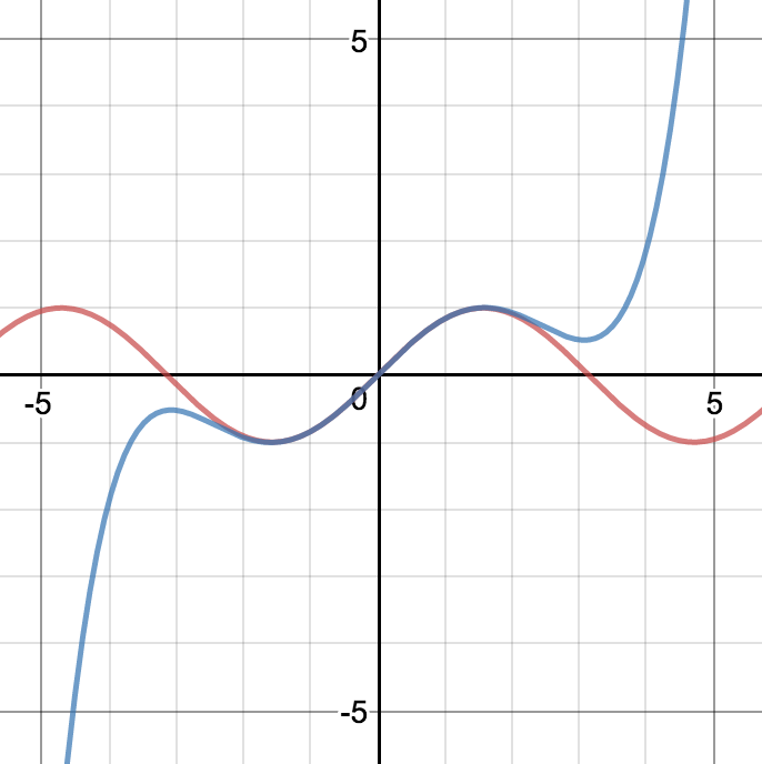
\[f(x) = a_0 + a_1x + a_2x^2 + \cdots + a_nx^n + R(x)\]

This is a reasonable assumption, because you’ve probably seen that polynomials can often be made to look like other functions. Here is a graph on which I’ve plotted $y = \sin x$ as well as $y = x - \frac{x^3}{3!} + \frac{x^5}{5!}$, which are the first three terms of the Maclaurin series for $\sin x$.

But I digress. Going back to our expression for a general function $f(x)$, all we have to do is find the values of our coefficients $a_0, a_1, a_2, \ldots, a_n$, and we will have our approximation. Well for starters, we can easily find $a_0$ because it is the constant term. If we substitute in $x = 0$, everything except that constant will disappear, so we can see that:

\[f(0) = a_0\]

A nice trick is that we can actually also use similar reasoning to find every other coefficient. How? By differentiating. Notice that:

\[f'(x) = a_1 + 2a_2x + \cdots + na_n x^{n-1}\]

Now, substituting $x=0$ will kill all the terms except $a_1$. Hence:

\[f'(0)=a_1\]

To find $a_2$, there is a slight difference. Note that $a_2$ was initially the coefficient of the $x^2$ term, so when we differentiate $a_2x^2$ twice we arrive at $2a_2$.

\[f''(0)=2a_2 \implies a_2 = \frac{f''(0)}{2}\]

We can repeat this process, differentiating as we go, to find $a_n$. Just to make this clear, let us examine do this step by step (but only consider the last term):

\[\begin{gather*} f(x) = [ \ldots ] + a_n x^n \\ f'(x) = [ \ldots ] + na_n x^{n-1} \\ f''(x) = [ \ldots ] + n(n-1)a_n x^{n-2} \\ f'''(x) = [ \ldots ] + n(n-1)(n-2)a_n x^{n-3} \\ \cdots \\ f^{(n)}(x) = n(n-1)(n-2)\ldots(3)(2)(1)a_n = n!a_n\\ \end{gather*}\]

So for our polynomial, we conclude that:

\[f^{(n)}(0) = n!a_n \implies a_n = \frac{f^{(n)}(0)}{n!}\]

Substituting these coefficients back into $f(x)$:

\[f(x) = f(0) + f'(0)x + \frac{f''(0)}{2!}x^2 + \ldots + \frac{f^{(n)}(0)}{n!}x^n\]

which completes our derivation of the Maclaurin series. If you want to find the Maclaurin series for a particular function, you just have to compute it’s nth derivative and substitute in $x=0$.

Conclusion for Part 1

I know that this is an abrupt end, and that I haven’t even started to explain the form of the gamma function, but in this post I showed that factorials have a natural relation to calculus, when one repeatedly differentiates a power of x. I trust that because of this, the reader may be getting a sneaking suspicion that there might actually be a link between factorials and integrals, which would explain why the gamma function looks the way it does.

In fact, there is a certain type of integration that does involve repeated differentiation. If you did A-level mathematics or an equivalent, you will almost certainly have come across it, though you may not see right now how it relates to factorials. I am referring to Integration by Parts. Head to Part 2 to find out more.