8-bit Julia set art in python

You may have heard a mathematician or physicist (or more likely your maths teacher) describe mathematics as beautiful. What could they mean by this? There is just something mysteriously attractive about the purity, complexity, interconnectedness, and underlying truth of it all (“Beauty is truth, truth beauty” - Keats). I can’t really say more than that, so I will leave you with a quote from the ‘man who loved only numbers’:

It’s like asking why is Ludwig van Beethoven’s Ninth Symphony beautiful. If you don’t see why, someone can’t tell you. I know numbers are beautiful. If they aren’t beautiful, nothing is. - Paul Erdős

But occasionally, mathematics can be beautiful in the traditional sense of the word.

What is this image, and how did I make it?

The Julia set

The Julia set is a type of fractal, a complex shape with a certain kind of evolving symmetry. What is interesting about fractals is that they are often based on very simple rules, which really begs the question as to where the dazzling intricacy comes into the picture.

While the Julia set comes in many flavours, we will consign ourselves to examine the easiest case, which is more than sufficient to produce pretty images; this is the Julia set defined by:

where $c$ and $z$ are complex numbers. To get from this equation to an image, we follow a relatively simple procedure

1. Choose a complex $c$ as the ‘seed’. This value of $c$ will determine the final picture, so choose wisely.
2. Draw a blank Argand diagram, i.e a set of axes with vertical being imaginary and horizontal being real.
3. Each point on this diagram is a complex number $z$. Repeatedly apply the above formula.
4. For each pixel, count the number of iterations it takes for the absolute value of the resulting complex number to exceed a certain limit. If it hasn’t exceeded this limit after a specific maximum iteration value, we terminate at this maximum.
5. Colour the pixel based on the number of steps it took.
6. Repeat this for all the points on the diagram.

Perhaps I have botched the explanation, but in essence, we count how many iterations of the above formula are required to increase $|z|$ beyond a certain bound, and colour accordingly. This is a remarkably simple procedure, and is rather easy to implement in python.

Python produces art

We will start by importing the necessary libraries. We need numpy for array manipulations, and matplotlib to produce our graphs (or art, if you prefer).

import numpy as np
import matplotlib.pyplot as plt
import matplotlib.cm as cm

In addition to deciding the resolution and the size of the plot, we must also settle the mathematical parameters. Firstly, we need a suitable $|z|$ to terminate the iterations; secondly, a value for the maximum number of iterations to compute. Quick experiments have suggested that values of 10 and 1000 respectively produce decent results.

# Resolution and plot size
x_res, y_res = 200, 200
xmin, xmax = -1.5, 1.5
width = xmax - xmin
ymin, ymax = -1.5, 1.5
height = ymax - ymin

# The mathematical parameters.
z_abs_max = 10
max_iter = 1000

You should definitely play around with some of the above parameters. In general, I left everything untouched except the resolution – I will demonstrate the effects of adjusting this later on.

x_res and y_res are the number of x and y pixels for which we will iterate the complex function. At some stage, we will have to loop over all of these pixels. But let’s first examine what happens for one pixel with coordinates (ix, iy).

We first map the pixel position to a point on the complex plane. ix ranges from 0 to 200, but our real axis ranges from -1.5 to 1.5. We thus have to ‘scale’ the ix range onto our Argand diagram.

real_part = ix / x_res * width + xmin
imaginary_part = iy / y_res * height + ymin
z = complex(real_part, imaginary_part)

This encodes the logic that we want to loop over all values between xmin and xmax, with increments of width/x_res. The same reasoning applies to the imaginary parts and iy.

Now that we have our $z$ and a $c$ (assuming the latter has already been chosen), we can proceed with the iterations. What I love about python is that the code practically speaks for itself – continue iterating as long as $|z|$ is smaller than our chosen limit, if we haven’t yet exceeded the maximum number of iterations.

iteration = 0
while abs(z) <= z_abs_max and iteration < max_iter:
    z = z**2 + c
    iteration += 1

So for each (ix, iy), we will have a certain value of iteration which should determine the colour. It will be easiest to implement the colouring if we first map all of the iterations to the domain [0, 1]. One shortcut for doing this is to just write:

iteration_ratio = iteration / max_iter

Because iteration is always greater than zero but less than max_iter, this value will be between zero and one, and will be proportional to the number of iterations it took to escape the $|z|$ circle.

All together now…

import numpy as np
import matplotlib.pyplot as plt
import matplotlib.cm as cm

# Parameters
x_res, y_res = 300, 300
xmin, xmax = -1.5, 1.5
width = xmax - xmin
ymin, ymax = -1.5, 1.5
height = ymax - ymin

z_abs_max = 10
max_iter = 1000


def julia_set(c):
    # Initialise an empty array (corresponding to pixels)
    julia = np.zeros((x_res, y_res))

    # Loop over each pixel
    for ix in range(x_res):
        for iy in range(y_res):
            # Map pixel position to a point in the complex plane
            z = complex(ix / x_res * width + xmin,
                        iy / y_res * height + ymin)
            # Iterate
            iteration = 0
            while abs(z) <= z_abs_max and iteration < max_iter:
                z = z**2 + c
                iteration += 1
            iteration_ratio = iteration / max_iter    
            # Set the pixel value to be equal to the iteration_ratio
            julia[ix, iy] = iteration_ratio

    # Plot the array using matplotlib's imshow
    fig, ax = plt.subplots()
    ax.imshow(julia, interpolation='nearest', cmap=cm.gnuplot2)
    plt.axis('off')
    plt.show()
    fig.savefig('julia_set.png', dpi=500)

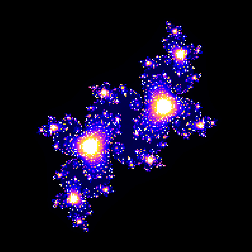
Running the code for $c = -0.1 - 0.65i$ gives the image at the top of this post.

Your turn

It is rather fun to play around with the different $c$ values. Here is a quick animation I made, using an adaptation of the above code:

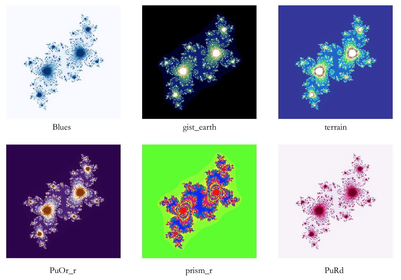
Or, if this colourscheme isn’t your thing, try playing around with the cmap parameter of imshow. Here is a list of the available colourmaps (for each one, you can append ‘_r’ to the cmap name to reverse the spectrum). I’ve shown a few different cmaps below:

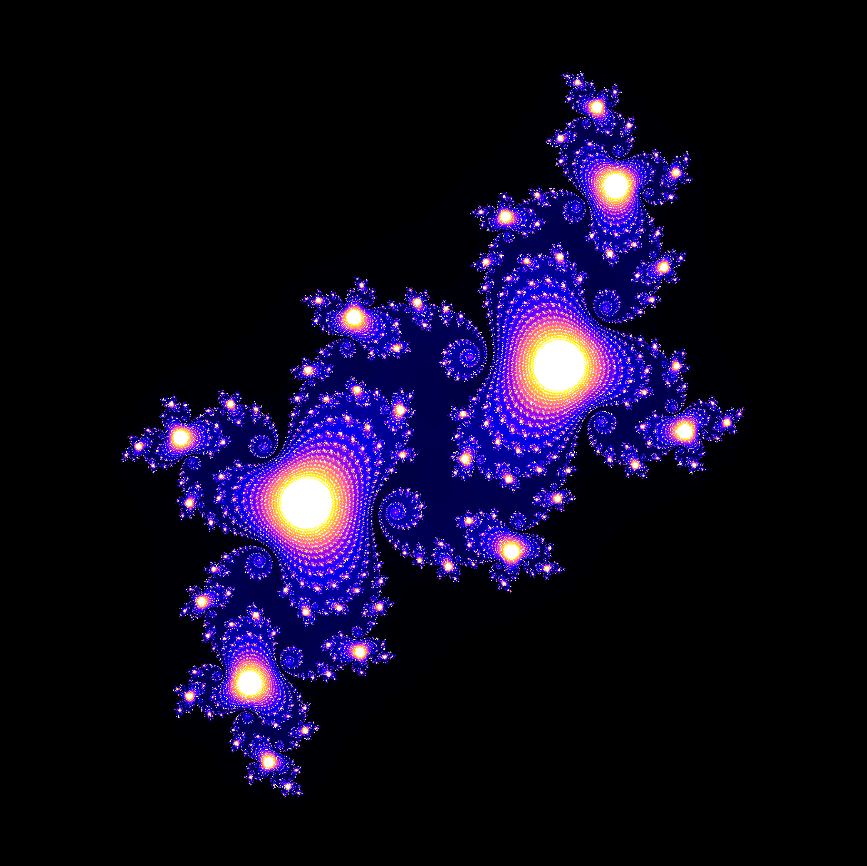
It is worth noting that the fractal we produced is actually infinitely complex. If you want to see some more of that complexity, try increasing the resolution. Be warned, though: the computation time grows as the square of x_res and y_res, so it might take some time to render. This is a render of the same initial image, except with the resolution set to 2000.

Conclusion

Clearly, this post doesn’t present the most efficient computation of a Julia set. For speed, we would use array manipulation rather than iterating over each pixel. However, the code is very easy to understand and we can still get some very pretty results.

There is a lot of room for personal preference: I have demonstrated the effects of choosing different c values, colourmaps, resolutions. However, you can even do stuff like ‘zoom’ onto a certain area of the fractal by changing xmin, xmax, ymin, ymax.

But my personal favourite is the image I showed you at the start of this post. That lovely rich purple combined with the 8-bit pixelation gives the image an other-worldly charm.

Play around with the code on GitHub to experiment some more. The code therein is very similar to what I’ve shown in this post, except I’ve also included the code to generate the animations and test different colourmaps.