A critical look at Greenblatt's Magic Formula
As the saying goes, when something sounds too good to be true, it probably is – all the more so when it comes to investing. In this short post, we look at the Magic Formula of Joel Greenblatt, as described in The Little Book That Still Beats the Market, critically examining the strategy and attempting to quantify its alpha.
What is unusual about this Magic Formula is that the person behind it is highly respectable. Joel Greenblatt is a value investing expert with an impressive performance track record; Gotham Capital’s persistent outperformance of the S&P500 speaks for itself. His book You Can Be a Stock Market Genius, despite the awful title, reignited my interest in discretionary stock picking and the chapter on spinoffs has led to some profitable picks. Consequently, this post is not seeking to debunk the Magic Formula, but rather qualify the claims made both by Greenblatt and the many investors who have since adopted it.
The supporting code is here, but it may not be much use on its own as it is intended to be run within the Quantopian research/algorithm environment.
How the Magic Formula works
The “Magic Formula” is a simple procedure to find good companies to invest in. It encompasses the philosophy that the ideal company needs to be high quality, and it needs to be cheap. That’s all there is to it.
There are many different ways these factors can be quantified, leading to several variations of the Magic Formula. Nevertheless, we will look at the canonical approach discussed in The Little Book that Still Beats the Markets. For the quality factor, Greenblatt uses the Return on Capital (ROC), which he calculates as the operating earnings (EBIT) divided by the total value of the fixed assets (property, plant, and equipment) and net working capital. By defining capital this way, instead of the more conventional sum of debt and equity, Greenblatt isolates the assets that are used to generate operating income. Hence, the ROC quantifies how efficient the company is at using its capital to generating earnings.
Cheapness is more straightforward. Greenblatt uses the ratio of operating earnings to the enterprise value (EBIT/EV) but you could instead use the earnings yield (inverse of the P/E ratio) or free cash flow yield. We should formulate the cheapness metric formulated as a yield, such that a higher quantity is better – this is useful when we are combining the cheapness rank with the ROC rank since both rankings will be in the same direction.
With this in mind, the overall procedure as suggested in The Little Book is as follows:
- Construct the universe of stocks: we require market capitalisations of more than \$100m and remove stocks in the Financials or Utilities sectors (since they have slightly different accounting).
- Calculate the ROC and the EBIT/EV
- Rank each company in the stock universe by ROC
- Rank each company in the stock universe by EBIT/EV
- Add the two ranks to get a combined score
- Each month, buy 2-3 positions from the top 20-30 companies
- Hold each position for one year (timing the sales/purchases for tax benefits)
The Little Book has a table showing the annual performance of the Magic Formula approach: from 1988 to 2004, Greenblatt claims that the Magic Formula returned an annualised 33% (compared to 14% for the S&P500). This is a phenomenal return – compare it with the scatterplot below showing the performance and track record of many famous investors:
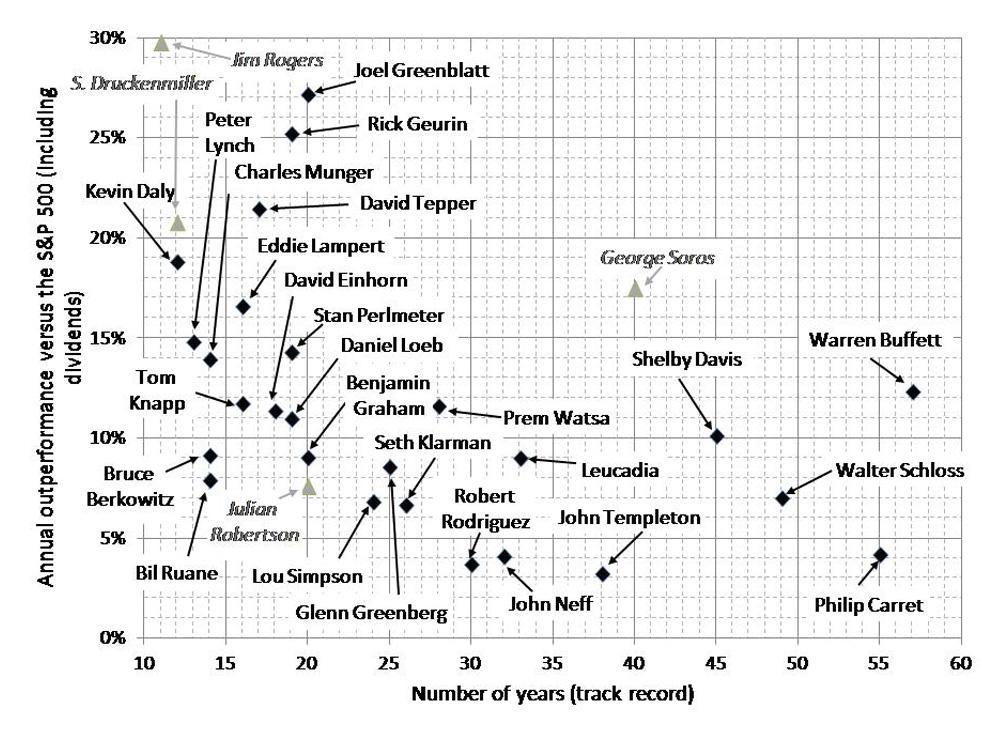
I certainly don’t suggest that Greenblatt has fabricated the results but it is difficult to believe that his simple procedure has consistently outperformed all these other superstar investors by such a large margin. In fairness, we do not have access to any other information about the strategy; those returns might be realistic (but less impressive) if they were achieved by taking twice as much risk.
Preliminary analysis of the ranking
Before running a full backtest, it is useful to start by analysing the information content of whatever signal we aim to capture. In the case of the Magic Formula, the signal is the combined factor score. Quantopian’s research environment (along with the excellent Alphalens library) is the ideal tool for the job – it’s incredibly well-suited to cross-sectional equity factors like this and is easy to pick up for someone with a bit of python experience. Below is a brief snippet of the core ranking logic:
# Filter sector and volume
sector = RBICSFocus.l1_name.latest
min_mcap = 100e6
sector_mask = (sector != "Finance") & (sector != "Utilities")
mask = (Fundamentals.mkt_val_public.latest > min_mcap) & sector_mask

# Quality
ebit = Fundamentals.ebit_oper_ltm.latest
ev = Fundamentals.entrpr_val_qf.latest
earnings_yield = ebit / ev
ey_rank = earnings_yield.rank(mask=mask)

# Cheapnesses
net_fixed_assets = Fundamentals.ppe_net.latest
working_capital = Fundamentals.wkcap_qf.latest
roc = ebit / (net_fixed_assets + working_capital)
roc_rank = roc.rank(mask=mask)

# Compute the score
combined_score = ey_rank / ey_rank.max() + roc_rank / roc_rank.max()
We can then feed this into a boilerplate function which computes the forward returns for each stock and creates a report on the predictive power of the signal. The fastest way to get an initial indication of the signal’s potential is to look at the quantile plot, which shows how stocks with the high ranking scores perform compared to stocks with lower ranking scores.
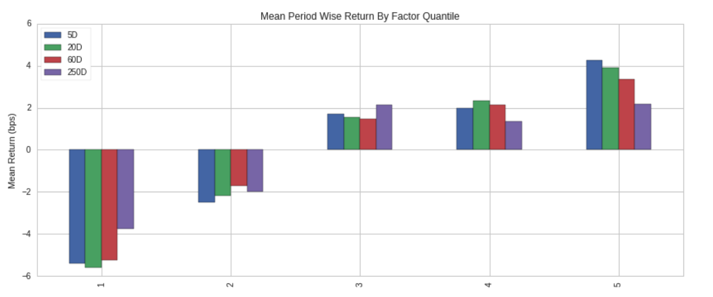
These quantiles are quite good; we see an overall monotonic increase, suggesting that high ranking scores are indeed associated with higher returns.
After the quantile plot, the next thing to look at is the information coefficient (IC), also known as the Spearman’s rank correlation coefficient, which measures the degree to which the ranking score is correlated with future returns. With a one-year time horizon, the Magic Formula score had a decent mean IC of 0.08. But rather than just looking at a point estimate of the value, it should be remembered that the predictive value of a signal may not remain constant with time. This is demonstrated in the plot below:
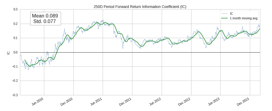
The Magic Formula score’s predictive power over a time period from 2004-2015 varied quite a lot, even becoming negative in 2009-2010. However, especially in more recent years, the Magic Formula has a robust IC.
As a brief interjection, you may wonder why we are only testing using data up until 2015. The reason is that in quantitative research it is vital to leave a few years “untouched” to act as the final validation step before you deploy a model live.
Overall, the results of this preliminary analysis are rather encouraging. With good quantiles and a reasonably high IC, the Magic Formula ranking does seem to have some predictive value. However, we shouldn’t get too excited; not all predictive signals are monetisable since the signal may not have sufficient magnitude to be profitable after transaction costs. The only way to find out is to run a proper backtest.
Backtesting the Magic Formula
For this backtest, we will follow Greenblatt’s procedure as closely as possible. Each month, we will pick the top two stocks according to the ranking (provided we don’t already own them) and allocate 1/24 of the total capital to each. After the first year, there will thus be 24 equally-weighted stocks in the portfolio. Each subsequent month will require us to liquidate the oldest two stocks to make room for two new entrants.
The only part of the Magic Formula we are not capturing is the tax optimisation – selling losers before the end of the tax year and winners at the start of a new one. For a fair comparison, we won’t consider taxes on the benchmark portfolio either. Quantopian’s default backtest includes transaction costs in the form of a 5 basis point (0.05%) slippage incurred every time a trade is made. The algorithm will have 100% turnover each year by design so the slippage should not be a major factor but it is good to incorporate it anyway.
Between July 2003 and December 2015, the Magic Formula strategy returned an annualised 11.4% (Sharpe ratio 0.60), versus 8.7% for the S&P500 (Sharpe ratio 0.54). This is clearly an outperformance of the benchmark (3% alpha) but by nowhere near as much as the Little Book claims.
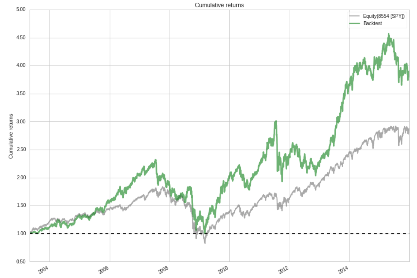
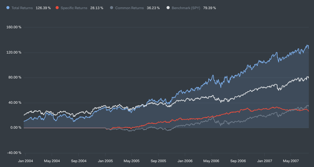
We can gain a more nuanced insight by considering different subsets of the backtesting period. Prior to mid-2007, the strategy was performing very well, achieving an annualised return of about 26% compared to about 18% for the benchmark – this is in line with Greenblatt’s claims. These returns are not just a result of taking more risk – notice the steadily growing specific return (the component of performance independent of the market’s movement, shown in red).
However, 2007-2010 tells a different story. The strategy had a drawdown of 57% (compared to 55% for the SPY), and the cumulative specific return went negative, meaning that despite the strong performance in the prior years, a “pure” (beta-hedged) version of the strategy would have lost money.
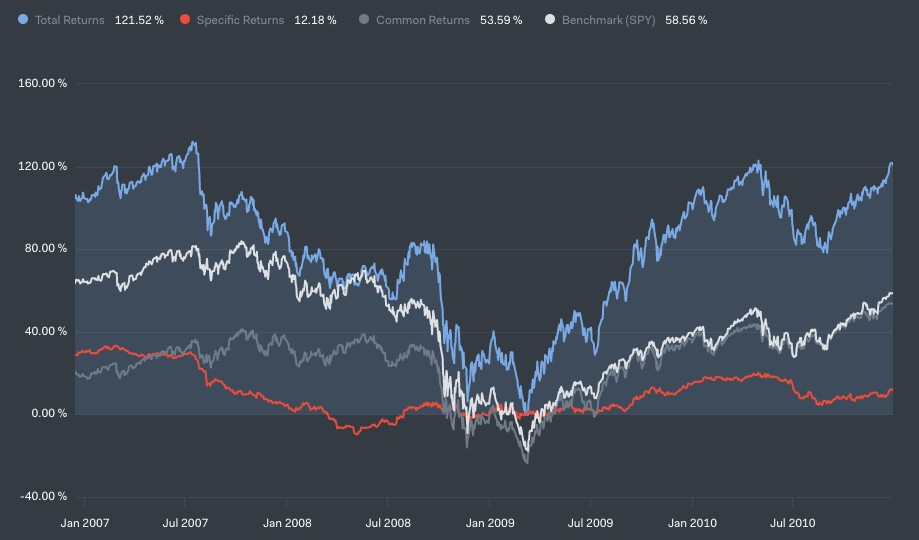
Post-2010, the strategy shared in the considerable market recovery, but its 12% annualised return was a slight underperformance of the benchmark’s 13%.
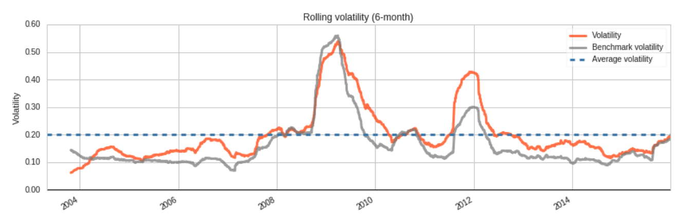
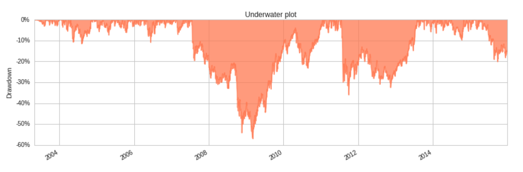
Over the backtest period, the Magic Formula was almost always more volatile than the market (which is to be expected since it holds only 24 stocks) and additionally had steeper drawdowns.
Improving the Magic Formula
Overall, the Magic Formula did indeed outperform the S&P500 between 2004 and 2015 but not by a large margin. For those of you who may be interested in building on top of the Magic Formula for your own investing, we now discuss some potential areas for improvement.
Composite factors: rather than using a single quantity to measure cheapness or quality, it might be better to aggregate different metrics, for example, earnings yield or FCF yield for cheapness. Jim O’Shaughnessy’s research in What Works on Wall Street suggests that a composite value factor is much more robust than single factors so we might have similar luck with quality and cheapness. As for the exact aggregation procedure, we could simply take the mean ranking across multiple different factors to start with but there is a lot of room here for sophistication – alpha combination can be seen as a portfolio optimisation problem so there is a large box of tools out there.
Trend: one danger with buying cheap assets is that there is nothing to stop them from getting cheaper. This could be mitigated using a momentum filter, only buying a highly ranked stock when we can see that it has positive momentum. Wesley Gray has done some interesting work in this area.
Long/short: if we believe that the Magic Formula score can identify both outperforming and underperforming assets, we can use a long/short basket strategy to hedge out market movement. The performance of this backtest should give a better indication of the quality of the ranking methodology compared to a long-only version. To make this more advanced, we can also consider hedging out various style exposures.
Before you boldly go forth testing these modifications, a word of warning. In the context of algorithmic trading, it is crucial to limit the number of backtests you run. What might seem like the “scientific” approach – running a backtest one at a time for each proposed modification to isolate its effects on performance – is poor practice because it can easily lead to overfitting and hence reduce the out-of-sample validity. To minimise this risk, a better approach is to sit down and carefully think about all the modifications you would like to make and ensure that you have a strong economic hypothesis behind each. For example, rather than carelessly adding a new fundamental factor (Quantopian has hundreds) you should argue why the factor should be predictive. If you later find out in a backtest that the signal is not predictive, or is predictive in the other direction, you should probably bin it.
I read an interesting discussion on the Quantopian forums where someone was trying to use the debt/equity ratio as a quality factor, with the hypothesis that a higher debt/equity ratio is associated with a lower quality company. The backtest looked great so it attracted a fair bit of attention but in a shocking twist it was revealed that there was a sign error in the code; in fact, a high debt/equity ratio was predictive of positive future returns. In this case, there is indeed a believable economic hypothesis to explain the observed effect – leverage amplifies returns (incidentally, this was a key point in Joel Greenblatt’s thesis on Host Marriott in You Can Be a Stock Market Genius) – but generally, you should be very careful about creating ex-post justifications for observed phenomena.
Conclusion
Based on our backtest, the surprising conclusion is that the Magic Formula is indeed a simple procedure that beats the markets on a risk-adjusted basis, with an annual alpha of 3% between 2003 and 2015. However, there are a couple of major caveats.
Firstly, the magnitude of outperformance is nowhere near what Greenblatt describes in The Little Book (33% vs 15%). This is likely due to the shift towards systematic equity ETFs over the past two decades, which arbitrage away inefficiencies like this. Furthermore, I hate to repeat the statement that “past performance is not indicative of future returns” but underlying this hackneyed phrase is the deeper concept of regime change. The performance of the Magic Formula in the post-crisis bull market was nowhere near as good as the performance in the 2004-2007 period; it is very possible that the 2008 GFC and subsequent central bank action represented a fundamental sea change, reducing the efficacy of certain value-oriented strategies. Hence, allocating capital to the Magic Formula strategy is implicitly making a bet that over your investment horizon, the market will be in a regime that rewards cheap high-quality companies.
Secondly, following the Magic Formula would still incur a significant psychological risk – the tendency for investors to let their emotions result in bad decision-making, for example, selling at the bottom of a crash or buying at the top of a bubble. It is very easy to look at the high annual return on a backtest and wish that you had used the strategy sooner, but would you really have been able to sit through a 56% drawdown like in 2008 without pulling your money out? Sure, in this case the market also experienced a great drawdown, but how about situations in which the market is going up but the strategy is losing money – in 2012, the Magic Formula strategy lost 5% while the SPY appreciated by more than 10%.
Although this post represents neither a confirmation nor dramatic refutation of the Magic Formula strategy, I hope that it at least provides a framework for investigating cross-sectional equity strategies and highlights some of the important pitfalls in backtesting.