Option-implied probability distributions, part 1

The key idea in Expectations Investing, a well-known book by Alfred Rappaport and Michael Mauboussin, is that to profitably invest in stocks one needs to find situations in which your view is variant to consensus expectations – a difficult task when you don’t know what consensus expectations are. There are several ways to figure out what the Street is thinking, the most common of which is to read sell-side research reports and get on the phone with analysts. However, earlier this year I wrote a post investigating how the current price of an asset can be used to infer implied expectations of future performance. In Part 1 of a two-part series, we look to extend this concept by examining what the pricing of option butterfly spreads can tell us about the implied expectations of the probability distribution of returns. Part 2 will consider a more advanced approach, closer to what is used by industry practitioners.

In writing this post, I have had to make a difficult decision regarding the level of background knowledge to assume; there is no escaping the fact that the subject of derivatives is highly mathematical. Therefore, in each section, I aim to present the intuition first and the mathematics second so the reader may decide how much of the mathematics they follow.

The supporting code for this post can be found in this Jupyter notebook.

Option prices are related to the distribution of underlying prices

A European call option gives you the right, but not the obligation, to buy an underlying asset (whose price at time t is denoted by $S_t$) at a particular date in the future (the expiry date, T), at a particular price (the strike price, K). If stock XYZ is currently trading at \$100 a share, one might think that an option to purchase it at \$120 next month is worthless. If the option were expiring today, that would be true – you wouldn’t want to buy something for \$120 when the current price is \$100. The option expiring next month, however, is not worthless because it’s possible that in the next month, the stock price could rise to \$130, in which case at expiry we could exercise the option and buy the asset at \$120 before selling it at \$130 for a neat \$10 profit.

We have established that this option is not worthless, which means that it has some value. Intuitively, its value is equal to the (present value of the) expected payoff at expiry. The payoff at expiry is the difference between the stock price and the strike price (\$130 – \$120 in the example above), or zero if the stock price is less than the strike price since you would not exercise the option. Hence, to value a call option C, we might write:

\[C(K, \tau) = e^{-r\tau} \mathbb{E}(\max[S_T-K, 0]),\]

where $\mathbb{E}$ is the expectation operator, $\tau \equiv T - t$ is the time period between now ($t$) and expiry ($T$) and r is the risk-free rate. $S_T$, the price at expiration, is a random variable – if we knew the future stock price with certainty life would be easy. The goal of this post is to find the probability density function (PDF) that describes $S_T$, which we will denote as $f(S_T)$; loosely speaking, this would tell us the probability that the stock trades near a certain price on the expiration date. With this in mind, to construct an expression for the expected payoff, we essentially need to sum the “probability that the stock price is $S_T$ at expiry” multiplied by the “payoff if the stock price is $S_T$ at expiry” for all possible $S_T$. This is done by integration since prices are assumed to be continuous:

\[C(K, \tau) = e^{-r\tau} \int_0^\infty \max[S_T-K, 0] f(S_T) dS_T.\]

We shall revisit this expression later on. For now, the key point is that there is a mathematical relationship between call option prices and the PDF of future returns.

A first approximation: option butterflies

As we established previously, the probability that the underlying stock will close at a particular price next month is somehow baked into the prices of options expiring next month. Intuitively, the price of calls should be positively related to the probability of an upside move – people would only want to buy an out-of-the-money (OTM) call, e.g. a call with strike \$120 when the underlying is trading at \$100, if there is some chance that their option will be in-the-money at expiration.

However, we cannot simply say that the probability of a certain price move is proportional to the price of call options with that strike because the price of a call embeds the expected profit from all expiry prices above the strike. In other words, the fair price of the K-strike option is related to the entire portion of the probability distribution above K, as the integral above demonstrates.

To proceed, we need to consider some combination of options that only profits if the underlying trades in a small range around a given strike at expiry. The price of such a structure would indeed be proportional to the probability of the associated price move. One such structure is the long butterfly, which consists of two short calls at a given strike combined with a long call at a higher strike and a long call at a lower strike, “bracketing” the strike of the short calls. The payoff diagram explains this better than I can:

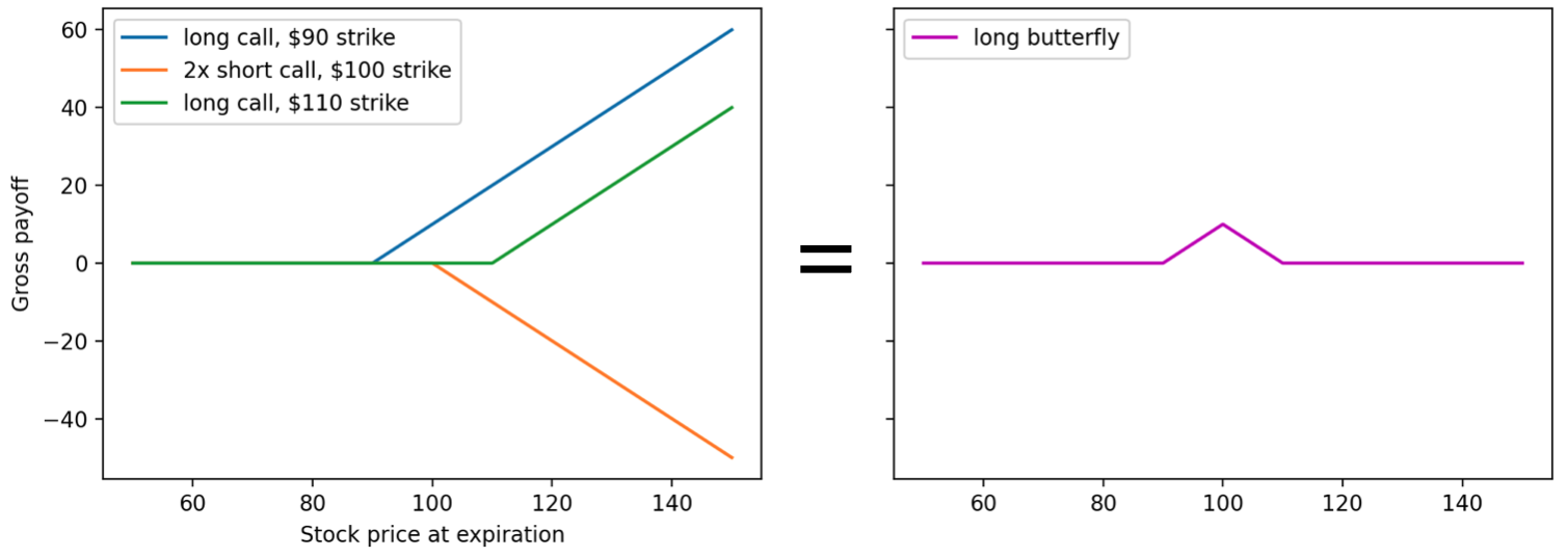
(Note that these payoff diagrams are shown on a gross basis – they have not been shifted down to account for the price of the structure).

The maximum payoff of a butterfly spread is equal to half the width of the spread (highest strike minus lowest strike). We shall denote the maximum payoff as $\Delta K$ – this payoff is realised when the stock price is equal to the central strike price at expiry.

Now, an important question. What is the fair price X of this butterfly spread?

Consider a biased coin which pays $\Delta K$ if the coin shows heads, which happens with probability p, and zero if the coin shows tails, which happens with probability $1-p$. The expected value of the coin toss is then $p\Delta K$. A rational individual who is neither risk-averse nor risk-seeking would pay exactly $p \Delta K$ to throw this coin.

We can apply the same reasoning to the butterfly, making the approximation that the payoff of the structure is either the maximum payoff $\Delta K$ or zero (i.e ignoring the sloped portion of the payoff function). In this case, requiring that the price of the structure is equal to the expected value of its payoffs, there is a simple relation between the maximum payoff of the structure $\Delta K$, the probability p that this maximum is received (equivalent to the probability that the price ends up at the central strike), and the price X of the structure.

\[p \Delta K = X \implies p = \frac{X}{\Delta K}\]

Let’s apply this to a real-life example. I downloaded some SPY option price data from my broker (about 3 weeks to expiration):

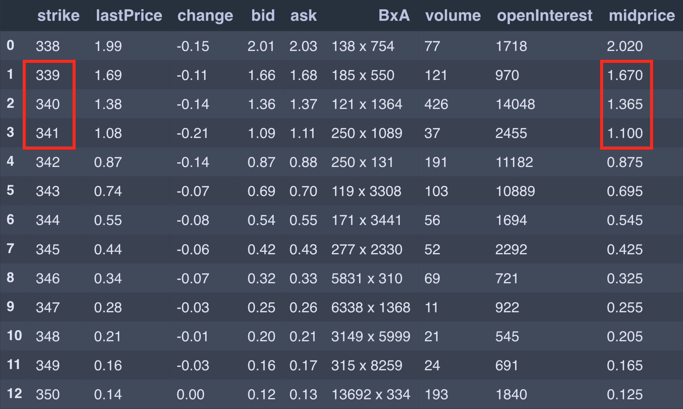
The probability that the SPY closes at \$340 on expiry (at the time of the snapshot, it was trading at \$332) will be approximated by considering the price of the 339/340/341 butterfly. For this structure, we have $\Delta K = 1$ and

\[X = 1.670 - 2 \times 1.365 + 1.100 = 0.04,\]

meaning that it would cost 4¢ to open this position (assuming we could fill at mid-market). Based on the formula derived above, the probability that the SPY closes at \$340 on expiry is $p = 0.04/1 = 4\%$.

In principle, we can now repeat this process for every possible butterfly to build out the entire distribution.

A kaleidoscope of butterflies

Unfortunately, there are several added complexities when working with real data. Let’s repeat the above calculation to find the probability that the SPY closes at \$349. The price of the 348/349/350 butterfly is

\[X = 0.205 - 2 \times 0.165 + 0.125 = 0.\]

Something is wrong here because we are receiving potential profits (with zero downside) for free! In an arbitrage-free market, this should not exist. Furthermore, the fact that the price of the butterfly is zero implies that there is no chance that the stock will trade at \$349 on expiry, which does not seem plausible, particularly because the same calculation tells us there is a 2% chance that the expiry price of the stock will be \$350.

This problem arises because of the illiquidity of some of the options contracts. There are far more people trading the \$350-strike option (because it’s a nice round number) than there are for the \$349-strike. Hence, for the latter, we cannot be certain that the price we see on the screen is reflective of the true price at which an order would be executed.

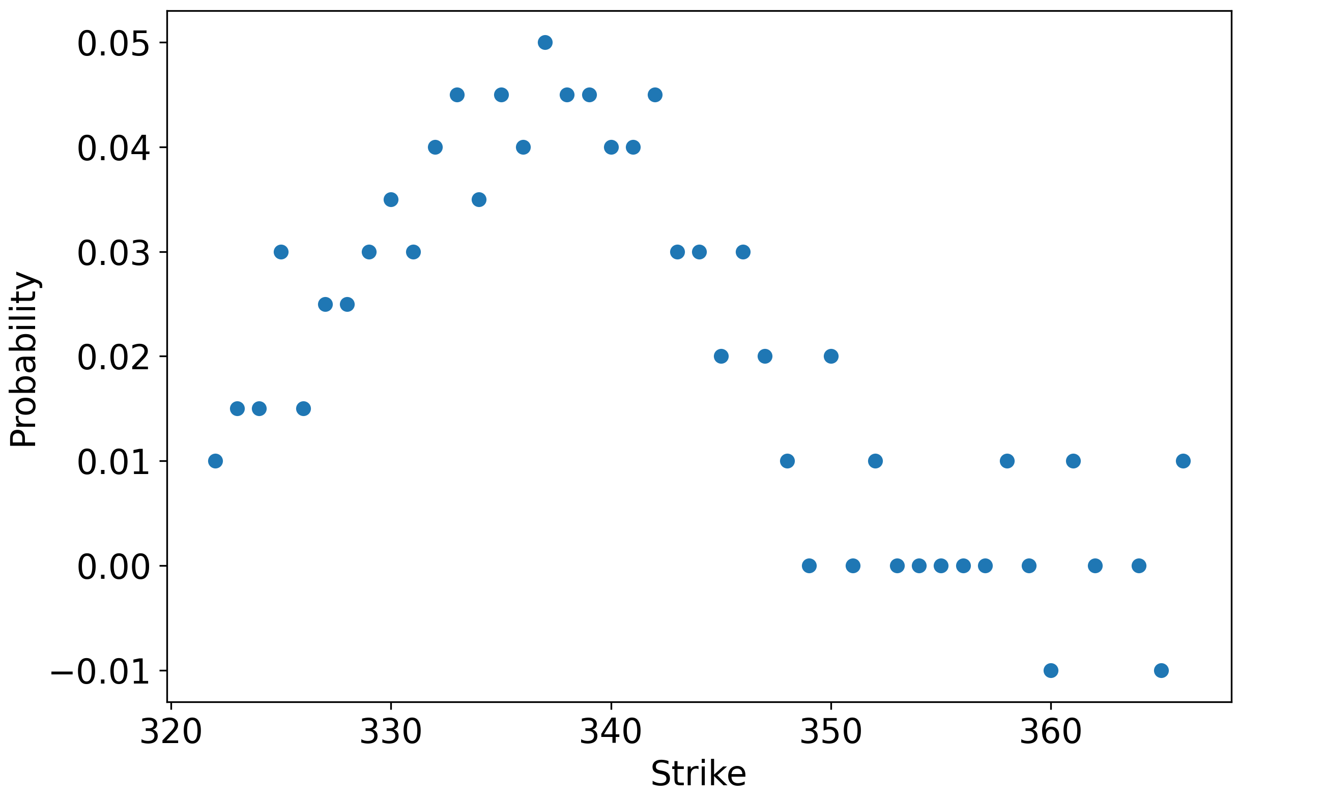
The plot below shows the butterfly-implied probabilities vary with the central strike price. Notice how noisy the data seems to be; there are even negative probabilities!

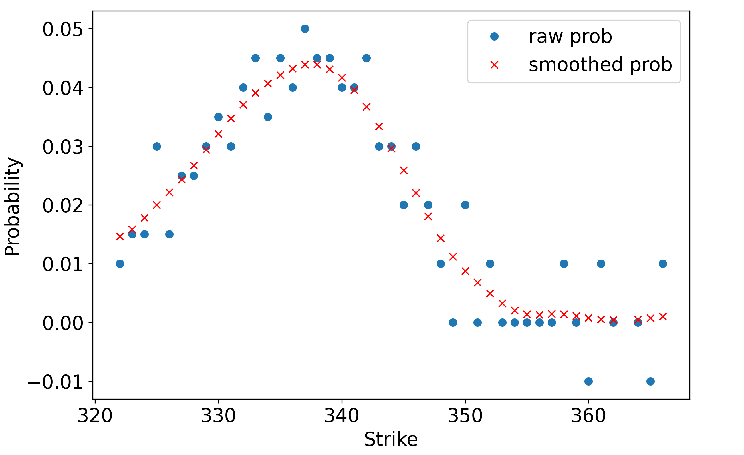
We need to clean this data up somehow. One approach would be to filter out the options with low volume, but that might result in us losing a lot of valuable data. Instead, I have decided to smooth the signal using a Gaussian filter. This works by convolving the noisy signal (in this case, butterfly-implied probabilities) with a Gaussian kernel – intuitively, each noisy data point is replaced with a weighted average of surrounding points (with weights determined by the Gaussian), resulting in a “blurring”. The result is clearly a major improvement:

We are not quite done yet, because all we have is a set of discrete points. We want a continuous PDF, so we need to interpolate between the points. To do so, we shall use a cubic spline, which fits piecewise cubic functions to the discrete points. This results in a relatively smooth PDF (indeed, by changing a parameter, we can decide exactly how smooth we want it to be):

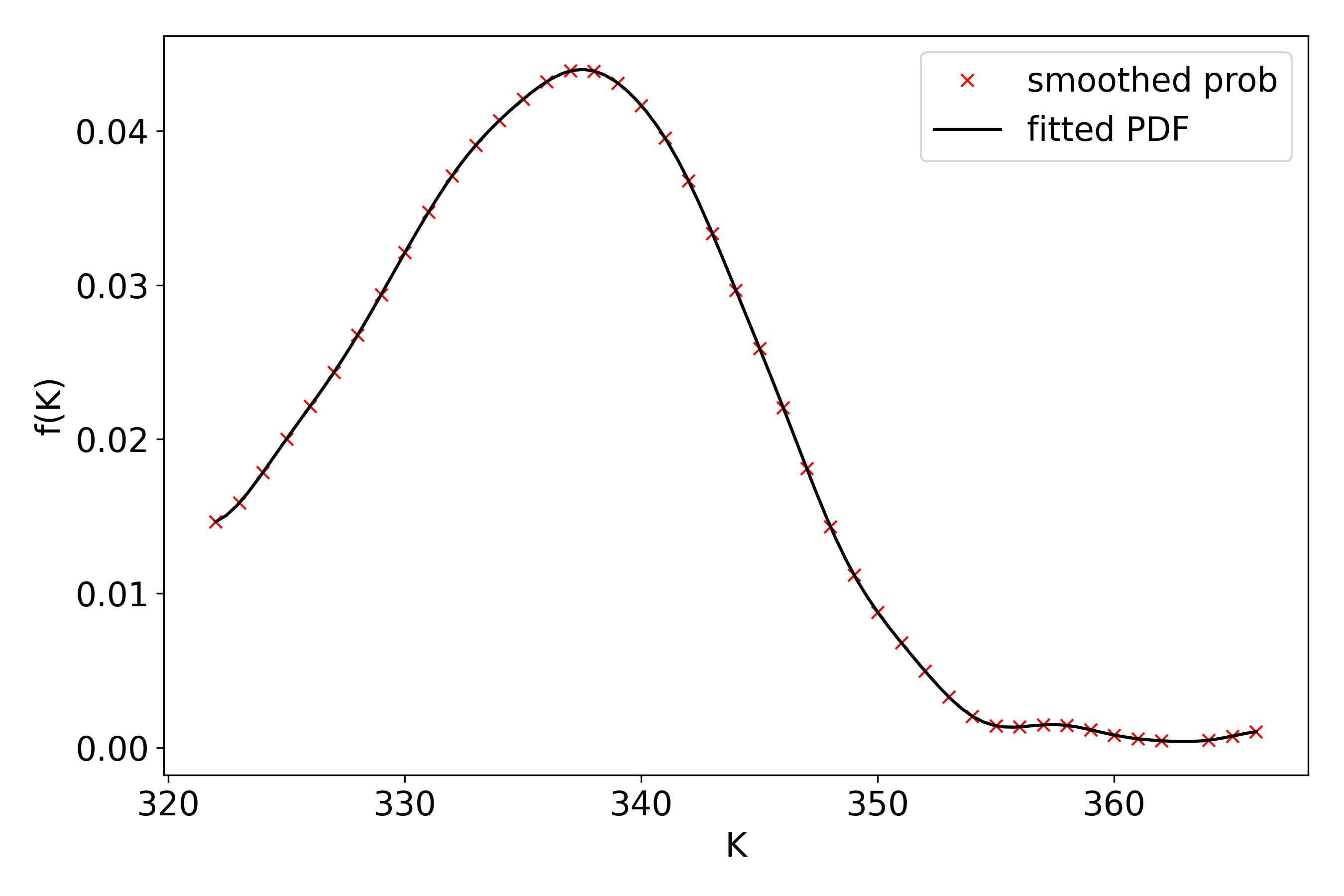
We have now managed to meet the objective of this post. We are now able to answer questions like “what is the probability that the stock trades above \$350 at expiry” by integrating the PDF.

The implied distribution of SPY prices has a characteristic log-normal shape, consistent with a bell-curve return distribution. This does not have to be the case. There are certain situations in which the return distribution can be highly asymmetric. For example, on September 13th Gilead announced that they would acquire Immunomedics for \$88 per share in cash, resulting in IMMU stock jumping up to near \$88. Once this happens, the probability of a move to the upside is low (though it could happen if a bidding war begins), while a downside move is definitely on the table – acquisitions may fall through for a number of reasons, be it antitrust, shareholder disapproval, or force majeure.

Conclusion

To sum up, the pricing of butterfly spreads can be a useful intuitive method for deriving the implied PDF of returns. That being said, the resulting distribution is not completely accurate, because it relies on the approximation that butterflies payoff in a binary manner. Furthermore, we have seen that dealing with real-life data requires several post-processing techniques to make the PDF “sensible”. In Part 2, we will examine a more sophisticated industry-standard approach to finding the option-implied PDF. Stay tuned!