Convexity in DCFs

In this post, we revisit classical DCFs through the lens of convexity. This leads to the counterintuitive finding that increased uncertainty about an asset’s fundamentals can sometimes be a good thing!

Overview of DCFs

DCF analysis is used to value cash flow generating assets. The key idea is that we prefer cash today to cash a year from now, such that £100 next year is only worth $£100 \nu$ to us today, where $\nu = 1 / (1+r)$ is the discount factor and $r$ is the discount rate (for $r > 0$ we have $\nu < 1$).

In a simple case, consider a perpetuity: an asset that pays out a fixed cash flow CF every year for eternity. Because of discounting, this is a geometric series with finite value: $V = CF / r$. If the perpetuity is growing, the value is still finite as long as the annual growth rate g of the cash flows is less than the discount rate. In this case, we have $V = CF / (r - g)$.

Unlike fixed income products, the cash flows for equities are not contractually determined; they depend on the uncertain profits of a business. A stock analyst must estimate DCF inputs like the cash flow growth rate. In practice, it’s easier to break down “cash flow” into more tractable components, the most important being revenue growth, operating margins, and capital expenditure:

\[\text{revenue} \times \text{op. margin} - \text{capex} = \text{free cash flow}\]

Analysts tend to input point estimates into DCFs but because of the difficulty of estimating inputs like the future revenue growth rate, I’ve often been intrigued by the idea of using distributional inputs instead, e.g. using a revenue growth rate of $30\% \pm 20\%$ rather than $30\%$.

This is not an original thought: there are tools such as Oracle crystal ball that allow you to construct a valuation distribution using distributional inputs. Aswath Damodaran, NYU’s “valuation guru”, often includes such analysis in his valuations (a good walkthrough can be found on his blog). Yet my impression is that analysts struggle to derive actionable insights from the resulting value distribution.

Sensitivity analysis – re-running the DCF with different inputs – is commonly used by equity analysts. But I think even in this case, emphasis is placed on the specific numbers (e.g. “if revenue growth is 20% instead of 30% my price target is \$12 rather than \$20) rather than the shape of the DCF function.

An investment puzzle

To motivate this exploration, let’s use a little puzzle.

Consider two cash-flow-generating private companies Aco and Bco. Assume that each has the following characteristics:

• Current cash flow is £10m/yr
• Cost of capital is 10%
• Each will have a high-growth phase for 10y, before settling down and growing at the rate of the overall economy (2.5% per year)
• We expect the growth rate in the growth phase to be 30%

The only difference between the two companies is as follows:

• We are very confident that Aco will grow at 30% per year
• But for Bco, while 30% is our expected growth rate, we are uncertain: we have identified two equally likely paths for the company, one in which the growth rate is 35%, and another in which the growth rate is 25%

Which company would we rather buy?

Perhaps intuition suggests that we take the relatively certain option, after all, uncertainty is normally a bad thing. This is wrong. At least in this simplified model of reality, Bco is a better choice. In the next section, we will do some arithmetic to illustrate this.

(If this feels wrong and the phrase “volatility drag” comes to mind, worry not: this point is addressed later on).

Two-stage DCF model

The setup of the problem invites the use of a two-stage DCF model, in which a cash-flow generating asset is modelled as the present value of future cash flows, with the cash flows being generated in two phases: a high-growth phase and a perpetuity phase (still growing, but at the same rate as the overall economy).

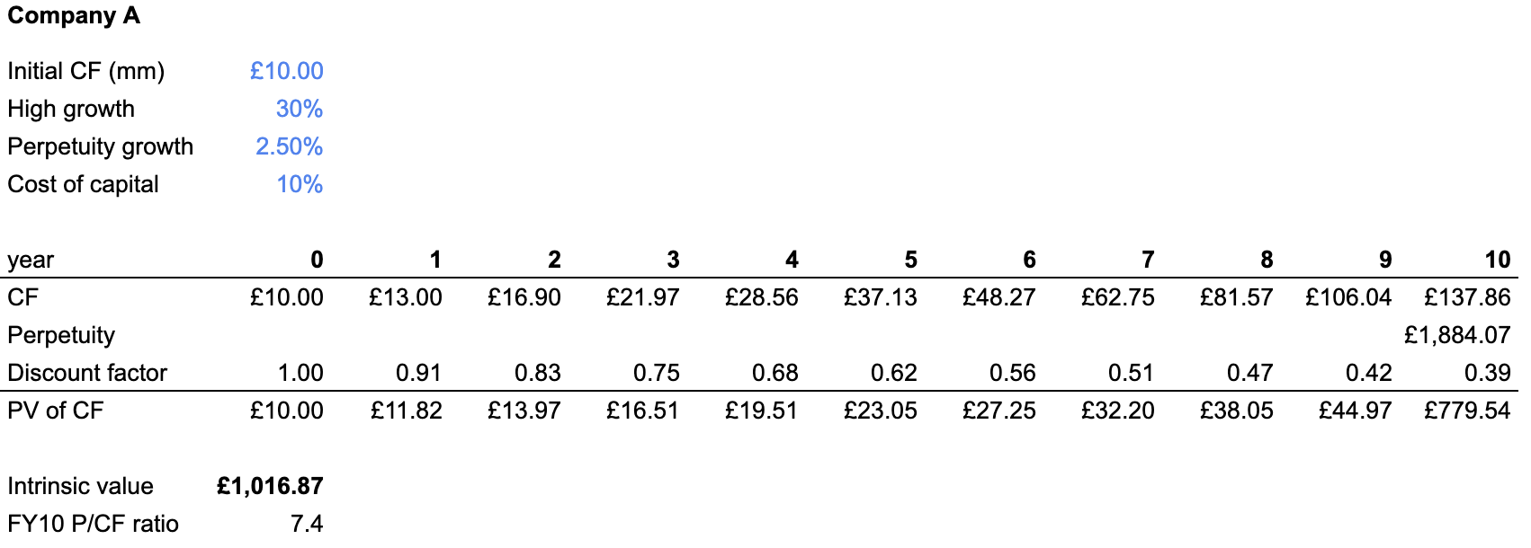
This is simple to implement in a spreadsheet: using the input assumptions from above, we find that the intrinsic value of Aco is £1.02bn. If this seems crazy for a company that only has £10m cash flow initially, remember that the cash flow is compounding at 30% over 10y.

For Bco, we run a DCF separately for the bad case (25% growth) and the good case (35% growth).

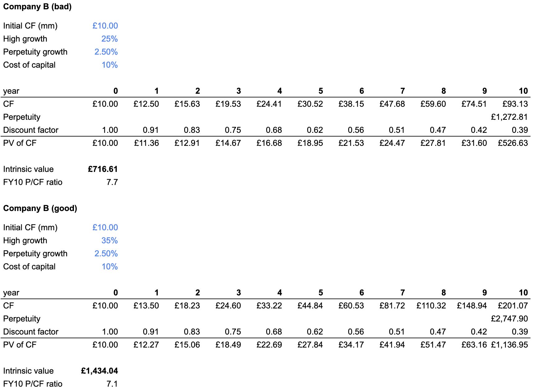
Because the good and bad cases are equally likely, the expected intrinsic value of Bco is simply the average of the intrinsic values in each case. But at this point we notice something strange:

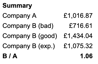
In expectation, Bco is 6% more valuable than Aco, despite having the same expected growth rate as Aco. For some reason, increased uncertainty in Bco’s growth rate has led to a higher expected intrinsic value!

DCF convexity

Uncertainty in the growth rate leads to a higher expected DCF value because the DCF formula is convex with respect to the growth rate.

Convexity

The high school definition of convexity: $f(x)$ is convex if its second derivative is positive, i.e. it curves upwards. An equivalent definition is that any straight line between two points is always above $f(x)$.

In a financial setting, $x$ is normally the price of some security (e.g. a stock price), and $f(x)$ is the value of some derivative contract whose payoff depends on the price of the underlying. For example, the plot below shows the price of a call option as a function of the underlying stock price (holding other inputs constant). The payoff diagram “curves upwards”, so the payoff is convex.

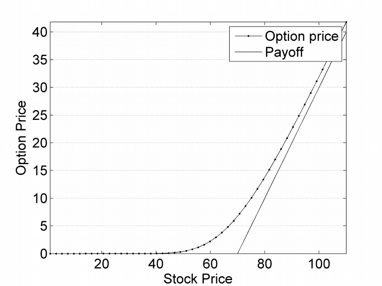
Yet the mathematical definition of convexity doesn’t entirely capture what traders mean when they talk about “convex bets”. Colloquially, a convex bet is one that “wins bigger than it loses”. Options possess convexity; they have limited downside (the premium you paid for the option) but potentially unlimited upside.

Stock prices go up and down a lot. The reason why options are “good” is that they make more money when the stock moves in one direction than they lose when the stock goes the other way. For example, we may have the following situation for a call option:

• Stock up 10%, option up 50%
• Stock down 10%, option down 20%

If you own an option, because of its convex payoff, you want uncertainty in the underlying. Considering the numbers above, given the choice between a stock that stays flat and a stock that goes up and down a lot, you would want the latter, because it “wins bigger than it loses”. This is why traders often say they are seeking convexity (though in reality what they mean is mispriced convexity – you have to pay to own an option’s convexity).

The main takeaway from this section: convex payoffs benefit from uncertainty/volatility. This is essentially the entire thesis of NNT’s Antifragile (my review and highlights here).

If you want to read more about convexity, I refer you to Kris Abdelmessih’s excellent post, which builds intuition and illustrates Jensen’s inequality.

The DCF formula

Because DCFs are almost always done in spreadsheets, you rarely see the DCF formula in the wild. Having written out the two-stage DCF formula below, I suppose that’s probably for the better:

\[PV = \frac{CF(1+r)}{r - g_0} \left[ 1 - \left(\frac{1+g_0}{1+r}\right)^{n+1}\right] + \frac{CF(1+g_0)^n (1+g)}{(r-g)(1+r)^n}\]

($CF$ is the initial cash flow, $g_0$ is the growth in the first stage, $n$ is the number of years in the first stage, $g$ is the perpetuity growth).

To show this is convex with respect to the growth rate, I could differentiate it twice with respect to $g_0$ and prove that the resulting expression is positive. That’s a lot of effort. Instead, here is a plot of the DCF value of an asset for different growth rates, fixing $CF = 10, r = 10\%, g=2.5\%, n=10$:

Note: the above analysis merely shows that the DCF formula is convex with respect to the growth rate. In principle, the DCF formula could be linear, concave, or convex with respect to the other value determinants. The plot below shows that DCFs are convex also to the discount rate, so uncertainty in the cost of capital is a good thing.

Is volatility good or bad?

The argument I have made so far can be summarised as follows:

• The expected value of a convex function increases with uncertainty in the input variable. In other words, convex payoffs like uncertainty.
• The DCF formula is convex with respect to growth rates.
• Hence, uncertainty in the growth rate increases the expected intrinsic value of an asset.

Another statement is also true: volatility in the growth rate decreases the expected intrinsic value of an asset.

How can it be that uncertainty in the growth rate increase the expected intrinsic value, but volatility in the growth rate decrease the expected intrinsic value?

Arguably there are some semantical shenanigans going on in my distinction between uncertainty and volatility, but there is an important point in how I laid out the puzzle at the beginning.

For Bco, the two equally likely outcomes are:

1. Fixed growth rate of 35% for 10y
2. Fixed growth rate of 25% for 10y

This is equivalent to saying that we flip a coin whose outcome determines whether we are in a universe where cash flows grow at 35% every year for 10y, or a universe where cash flows grow at 25% every year for 10y. Critically, once the universe has been chosen, there is zero volatility in the cash flow growth rate.

Now consider a modified puzzle, where we choose between:

• Aco: as before, cash flows grow 30% every year for 10y before entering perpetuity growth.
• Cco: cash flows grow at $30\% \pm 20\%$, i.e. every year we draw the growth rate from a normal distribution $N(30\%, 10\%^2)$.

To value Cco, we can’t simply draw growth rates from the normal distribution and substitute them into the DCF formula (this is the whole point!): we must simulate different paths and calculate the DCF value of each path, before taking the mean across all paths.

The below chart shows how the expected intrinsic value of the asset varies with the volatility of the cash flow growth rate:

We can see that volatility in the growth rate (slightly) reduces the expected intrinsic value of the company.

This phenomenon is closely related to variance drag – mathematically, for growth rates drawn from a normal distribution $N(\mu, \sigma^2)$, the expected CAGR (geometric mean growth) is $\mu - \frac 1 2 \sigma^2$. This concept is nicely explained in one of Benn Eifert’s classic tweet threads. The situation is not quite the same as the typical variance drag setup because we are not considering the compounding growth of an investment: in particular, we are not saying that the company’s NPV is growing at a compounding rate, only its cash flows.

To summarise, we need to make the subtle distinction between an uncertain cash flow growth rate and a volatile stream of cash flows. Because of convexity, the former is good. But because of variance drag, the latter is bad. In real life, both will show up at the same time and pull in different directions!

Conclusion

The main lesson of this post is that you should pay attention to convexity because it turns uncertainty into increased expected value. When you own a convex payoff, you want uncertainty in the input parameter!

For equity analysts reading this, a more tangible takeaway is as follows: if you can see a credible blue-sky scenario for a company (e.g. a scenario that leads to a much higher growth rate or lower cost of capital), because of the convexity of DCFs, that blue-sky scenario might be so accretive to the intrinsic value of an asset that the bear case is irrelevant.

More generally, this post is a teaser for the type of insight that can be gleaned when we start considering distributional inputs to DCFs. I’m fascinated by the idea of using old tools in new ways and hope to explore other aspects of “probabilistic valuation” in future posts.