Statistical arbitrage in closed-end funds

Sometimes, it is cheaper to buy a basket of assets than it is to buy the assets in the basket. In this post, we discuss closed-end funds and why they often trade at a discount to their net asset value. Furthermore, we explore whether this could be the basis for an algorithmic trading strategy.

Closed-End Funds vs ETFs

Most of us are probably familiar with exchange-traded funds (ETFs) – baskets of securities where the basket itself is tradable. The ETF industry has grown rapidly over the past few decades because ETFs provide a low-cost way to get exposure to a certain market, sector, or strategy.

In this post, we will instead be discussing closed-end funds (CEFs). On the surface, these may seem similar to ETFs: CEFs are also baskets of securities, and they can also be listed and traded on an exchange. A pedant might point out that by definition, a CEF is an ETF since it is a fund that trades on an exchange – this is unfortunately not correct, as there is a true conceptual distinction.

We often like to think of ETFs as upscaled equivalents of a personal trading portfolio. One gives money to a manager, who in return issues a share of the ETF to represent the ownership and invests that money in a basket of assets. This mental model is, in fact, a much better description of CEFs. ETFs are a little bit more complicated. For both ETFs and CEFs, an important point is that the share price is not “naturally” guaranteed to be equal to the value of all of the securities that the fund owns, i.e the net asset value (NAV). This is because the share price of the fund is determined by supply and demand – if everyone in the world suddenly wants to buy the shares of a fund, the share price can shoot up independently of the value of the underlying assets. However, ETFs have an interesting mechanism for ensuring that these deviations between the price and NAV are very short-lived.

ETF fund managers are seldom the people who buy and sell the securities. They instead turn to authorised participants (APs), typically investment banks, who transact in the underlying securities. The fund manager then issues shares of the ETF to the AP, in return for the securities that were bought. This process is known as creation because shares of the ETF are being issued. The AP is then free to hold these shares, or more often, trade them on a stock exchange. However, the AP’s role goes far beyond the initial purchase of the securities to set up the ETF. They play a critical role in ensuring that the ETF share price never strays too far from the NAV. Any momentary supply-demand imbalances can be arbitraged away – for example, if there is suddenly less demand for the ETF, and it trades at a discount to the NAV, the AP can buy ETF shares on the open market and redeem them from the ETF fund manager. This locks in an arbitrage profit and drives the ETF price back towards the NAV.

This is why ETFs are open-end funds: the fund manager can issue/redeem however many shares they want. Conversely, CEFs issue a fixed number of shares when they first IPO, and there is no subsequent creation or redemption. As a result, we might expect there to be a larger spread between the CEF price and the NAV (compared with an ETF’s price and its NAV).

NAV Arbitrage and the Closed-End Fund Puzzle

Although CEFs don’t have the same creation and redemption mechanism as ETFs, there is still a fundamental link between the NAV and the price.

Let’s take a very simple case where we have a “basket” of two stocks, say AAPL and FB. As of the time of writing, AAPL has a price of \$289/share and FB has a price of \$202/share. The fair price of this basket is then $\$289 + \$202 = \$491$. This is intuitively obvious, but to drive home the point, we can ask what would happen if the basket weren’t priced at \$491. If the basket was instead trading at \$400, we would be correct in thinking that the basket is “cheap” – we’d certainly rather buy the basket than the two stocks individually. We can take this a step further and go long the basket and short the individual stock, which results in a risk-free profit once other market participants realise that the basket and the two stocks should be priced identically.

If we are a majority shareholder in the fund, we don’t even have to rely on the rationality of other market participants; we can force a liquidation event, in which the fund manager sells all the securities, distributes the proceeds as dividends, then delists the shares. At such a time, the price of the shares must be equal to the NAV, less the cost/slippage from selling the securities.

Thus, even without APs, the price of a CEF should track its NAV. However, empirically, this is not the case. Below, we show the price vs NAV for two large funds, the Eaton Vance Global Diverse Equity Fund (EXG), and the Aberdeen Asia-Pacific Income Fund (FAX), using data from CEFConnect:

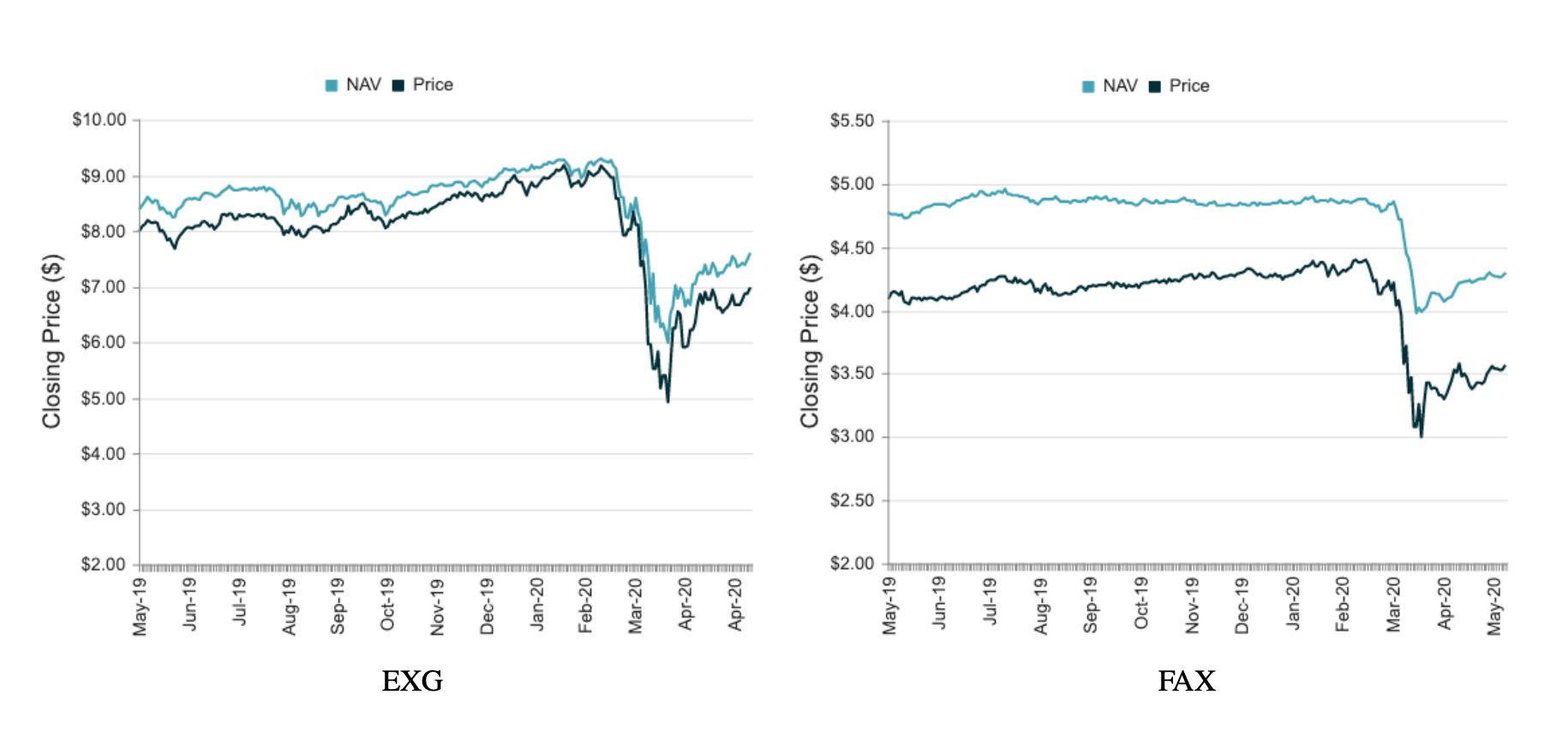
For both of these funds, the share price trades at a persistent discount to the NAV – in the case of FAX, this discount is almost 20%. The existence of this spread (typically a discount) between the price and the NAV is known as the Closed-End Fund Puzzle.

There are several responses to the closed-end fund puzzle, though I would refer interested readers to Lee, Shleifer and Thaler (1991) for a detailed investigation:

• Cost of transacting – we already touched on this. In a liquidation event, we will not receive the full NAV because of the transaction costs, which may be rather significant if we are dealing with assets that are hard to sell. We can verify that this is indeed a contributing factor by observing that there seems to be a broad negative correlation between asset liquidity and the spread. Equity CEFs typically have a smaller discount compared with bond CEFs, because equities are easier to sell.
• Difficulty of arbitrage – in practice, it is hard to lock in a risk-free arbitrage because it may be very difficult to transact in the underlying (which is sometimes why the CEF was created in the first place). Furthermore, the fund managers are free to enter and exit positions as they desire, so an arbitrageur would have to constantly make changes to adequately replicate the portfolio.
• CEFs have a much lower fraction of institutional ownership than the underlying – it is possible that the pricing of CEFs is less rational as a result, with price movement driven by liquidity and sentiment rather than value.

The rest of this post will investigate the hypothesis that the spread between the CEF price and its NAV is mean-reverting, or more intuitively, that larger discounts are predictive of a future price increase and larger premiums are predictive of a future price decrease.

Statistical arbitrage

Statistical arbitrage (stat arb) is a fancy term describing the process of buying assets that are statistically cheap and selling assets that are statistically expensive, hoping to lock in the difference. The key is that these arbitrage opportunities are not at all risk-free, they are only really arbitrage opportunities in the sense that if we make a sufficiently large number of such bets, we will have a positive expected value (the law of large numbers).

The classic stat arb strategy is pairs trading, which involves finding two assets that are highly correlated and trading the spread between them. The standard example is Coca-Cola and Pepsi. Rather than making a bet on the overall direction of either stock, we can eliminate idiosyncratic risk by trading the difference between the price of Coca-Cola shares and Pepsi shares. To ensure that our correlations aren’t spurious, it is desirable for there to exist some fundamental economic reason why the two assets are related. In the case of Coca-Cola and Pepsi, the argument goes that because they are essentially substitute goods, any widening of the spread should be temporary. So if Coca-Cola stock appreciates while Pepsi’s stays flat, the statistical arbitrageur may long Pepsi and short Coca-Cola.

Stat arb is most effective when the spread is stationary, a technical term which describes the fact that the data-generating process for the time series does not change (its statistical properties are constant in time). This is a logical requirement – if the statistical properties were changing, nothing stops the spread from widening forever. Stationary series, as a consequence of the definition, are almost always mean-reverting – wider spreads are more likely to be followed by narrower spreads and vice versa.

In many ways, the spread between the price and NAV is the ideal candidate for a stat arb strategy. There is an incredibly strong economic link between the NAV and the price; we even know that at liquidation they must converge (less fees). The only wrinkle is that the NAV isn’t actually a tradable security. This doesn’t completely preclude the development of a trading strategy, but it wouldn’t be a proper pairs trade since we would only be acting on one of the legs. For example, if the CEF were trading at a 20% discount to NAV, a pairs trade would involve going long the CEF and “short the NAV”. In this case, even if both the NAV and the price of the CEF decrease, your position would be fine because the short side hedges you. But since you can’t trade the NAV, although you are still able to make bets on convergence (by going long the CEF when it is trading at a discount), such bets would not be pure bets on the spread.

It may be possible to work-around this by computing the beta of the NAV with respect to a comparable asset/ETF then trading the correct amount of that comparable. For example, if we were dealing with a CEF that invests in high yield bonds, we could compute the beta of the NAV to a high yield bond ETF (e.g. HYG). Let’s say $\beta = 2$, in which case we could bet on the spread converging by going long \$10k in the CEF and short \$5k of HYG. But again, this is not a perfect bet on the spread.

This important caveat notwithstanding, we shall now examine the stationarity of the price-NAV spread and investigate whether the spread is predictive of future returns.

The price-NAV spread

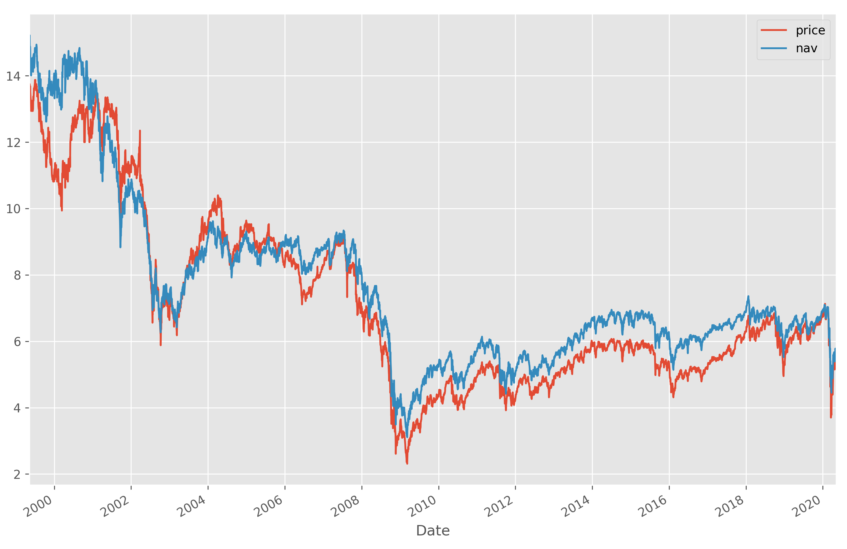
We will look at a single CEF, namely, the Liberty All-Star Equity Fund. This was chosen because it is large and liquid (and has a memorable ticker, USA). Using an appropriate colour scheme, we can plot the price and NAV:

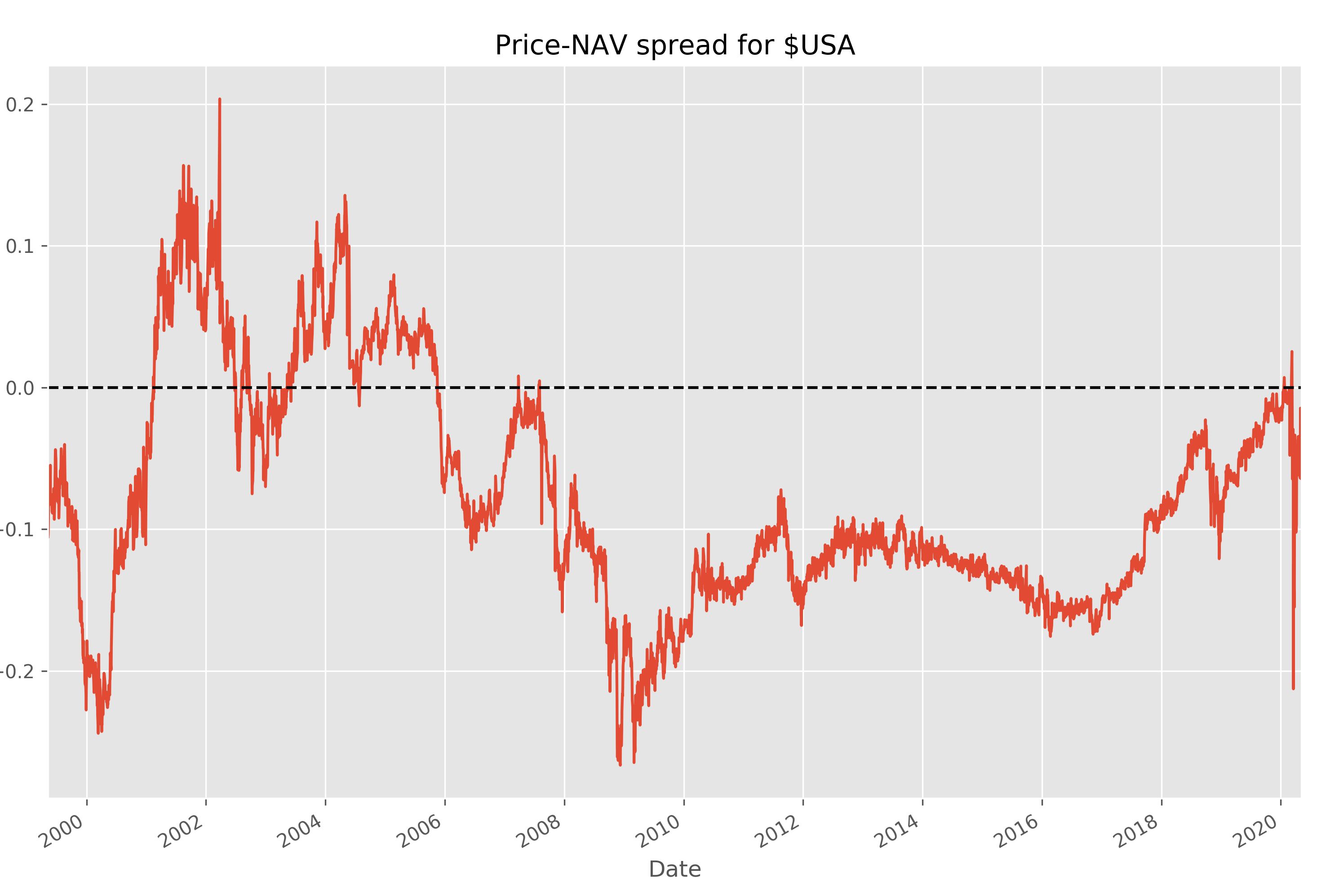
From 2000 to 2009, the CEF alternates between trading at a discount/premium to NAV, before settling into a persistent discount from 2009 onwards. Below is a plot of the spread, i.e $\text{price}/\text{NAV} - 1$ (positive is premium, negative is discount).

Now, we can perform an Augmented Dickey-Fuller test to determine whether the spread is indeed stationary. It turns out that although there is not enough statistical evidence to reject the null hypothesis that the spread is non-stationary, the price and NAV are significantly cointegrated (this intuitively means that some linear combination of the price and NAV is stationary).

Stationarity aside, let’s press on with a somewhat crude estimate of the predictive value of the spread. Rather than doing any kind of proper backtest, we will just compute the correlation between the current spread and the subsequent change in the spread. To be specific, we shall use the Spearman rank correlation coefficient, sometimes referred to in finance as the information coefficient (IC), which is more robust to nonlinearity than the Pearson product-moment correlation coefficient.

We find that the correlation between the current spread and the change in the spread over the following week is $-0.06$ (statistically significant at the 5% level). It is comforting that there is a negative sign because it supports the hypothesis that the spread mean-reverts: premiums are correlated with decreasing premiums, discounts are correlated with narrowing discounts.

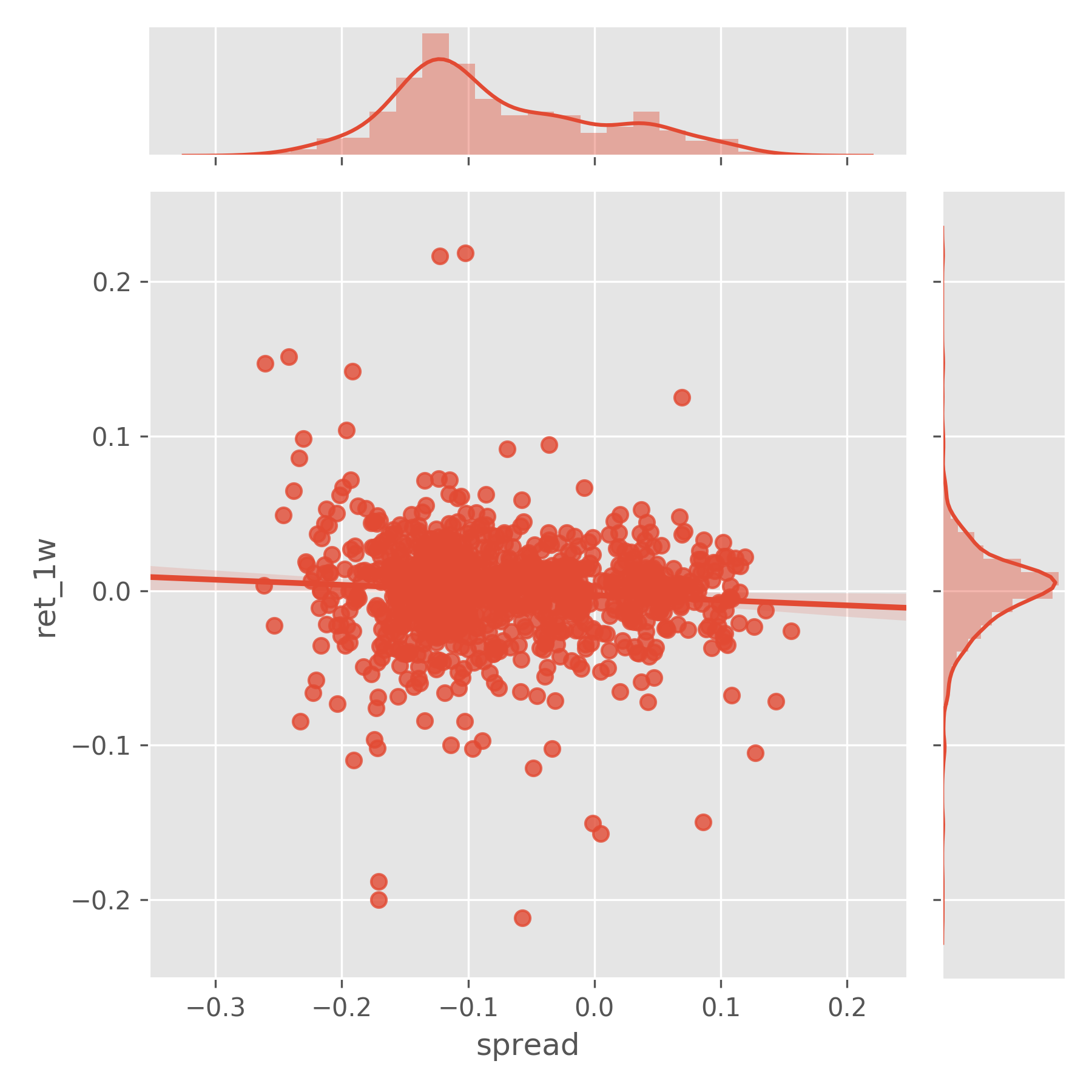
However, as we discussed previously, the NAV isn’t tradable so we instead want to find out the correlation between the current spread and the price return of the CEF. The same Spearman rank calculation gives a correlation of $-0.07$. This is quite a decent IC – according to a paper by JP Morgan Equity Research, investors can “achieve significant risk adjusted excess returns with information coefficients between 0.05 and 0.15” (the sign doesn’t matter here). We can visualise the relationship with a scatterplot:

Conclusion

There is clearly a lot more exploration that needs to be done – we have only looked at the spread for a single fund, and have chosen a simplistic information coefficient analysis rather than conducting a full backtest. Nevertheless, the results thus far have been quite encouraging. In addition to the reasonably high information coefficient, we have a clear economic hypothesis about why the discount to NAV may be a persistent predictive factor. In a recent MacroVoices podcast, Eric Peters shared a great insight (emphasis is mine):

Our approach to anything that we ever do in markets, is to first ask the question: why do you get paid to do something?

Without this economic understanding, it’s much more likely that any pattern you’ve discovered is a statistical spectre that haunts the historical data but will disappear in the daylight of future data.

To answer the question in the introduction, I do think that this could form the basis of a trading strategy and hope that over the next few weeks I will have a chance to investigate further.