Hypothesis testing in quant finance

At its core, science is about making falsifiable hypotheses about the world (Popper), testing them experimentally, then using the experiment outcomes to refute or refine the hypotheses. The scientific method is an integral part of quantitative finance; it provides a framework we can use to identify and analyse trading signals or anomalies.

In this short post, we discuss a general method for hypothesis-testing in finance, using Monte Carlo simulations to compute the probability that an observed signal can be explained by random chance.

This post is an expanded version of a Twitter thread I wrote. The supporting code can be found in this notebook.

Hypothesis testing and p-values

As a necessary prelude, we first discuss a somewhat controversial topic: the p-value.

Wikipedia defines the p-value as:

the probability of obtaining test results at least as extreme as the results actually observed, under the assumption that the null hypothesis is correct

With a definition like this, it’s no surprise that p-values are so widely misinterpreted. We can try and understand the intuition behind p-values by considering an example.

Let’s imagine that we want to find out whether some new teaching method X (e.g. forcing students to make flashcards) improves test scores versus the default method Y. A simple approach is to split the cohort of 100 students into two groups, making 50 of them do X and the other 50 do Y. We can then compare the average score between the two cohorts.

The problem arises when we try to interpret the results. If the X students had an average grade of 70%, while the control group had an average of 60%, did X really improve test results or was it a random fluke? How about if it was 60.1% vs 60.0%? Or 80% vs 50%?

This is where hypothesis testing comes in. We set up a null hypothesis and test whether there is sufficient evidence to reject the null hypothesis. In our example, the null might be that there is no difference between the mean scores of the X and Y groups.

To test this, we assume that the null hypothesis is true – that X doesn’t actually improve test scores – and compute the probability that we would see X have an average score of 70% vs the control group’s 60%. This probability is the p-value.

At the risk of being imprecise (and thereby perpetuating the misinterpretations of p-values), I think of the p-value as the probability that random data can explain your results.

The trouble with p-values

One of the major criticisms with p-values is that they answer the wrong question. We aren’t truly after “the probability that random data can explain your results”. We actually want to know the probability that X causes test results to improve, given the observed data. To answer questions like this, a different box of tools is needed – I’d highly recommend Judea Pearl’s The Book of Why if you’re interested in learning more – but for now we will proceed under the assumption that the p-value is indeed a statistic of interest.

Even then, there is a subtle issue that we glossed over above. The p-value can only be calculated if we assume that the quantity of interest is drawn from a particular probability distribution. In our example, we can’t actually “compute the probability that we would see X have an average score of 70% vs the control group’s 60%” unless we make some assumption about the distribution of test score (typically a normal distribution or t-distribution is used).

In finance, these types of assumptions rarely hold. Furthermore, we are often looking to test more complicated hypotheses, such as “this time series is stationary” or “this data is normally distributed”. You might be lucky enough to find that someone has already figured out how to test a particular hypothesis – for instance, the augmented Dickey-Fuller test can be used to test for stationarity and Jarque-Bera for normality. But generally, properly calculating p-values is hard!

The good news is that we often don’t need to properly calculate a p-value. Monte Carlo simulations can give us “quick and dirty” estimates of the p-value that might be good enough.

Case study: ETF seasonality

I came across a tweet from Mitchell Rosenthal in which he observes that the iShares Singapore ETF (ticker EWS) shows positive returns in 89% of April months from 2002-2020. This seems like an interesting anomaly, but with only 19 Aprils, it certainly seems plausible that this anomaly could be generated by random chance alone (remember: the probability of this is quantified by the p-value).

Firstly, let’s replicate his findings. I downloaded data for the EWS ETF going back to 1996 and calculated how often each month had a positive return.

def compute_pct_up_months(df):
    # df is a dataframe of daily close prices
    df_mth = df.resample("M").last()
    month_up = df_mth.pct_change().dropna() > 0
    pct_up = month_up.groupby(month_up.index.month).mean()
    return pct_up

A bar chart showing the fraction of up-months is shown below:

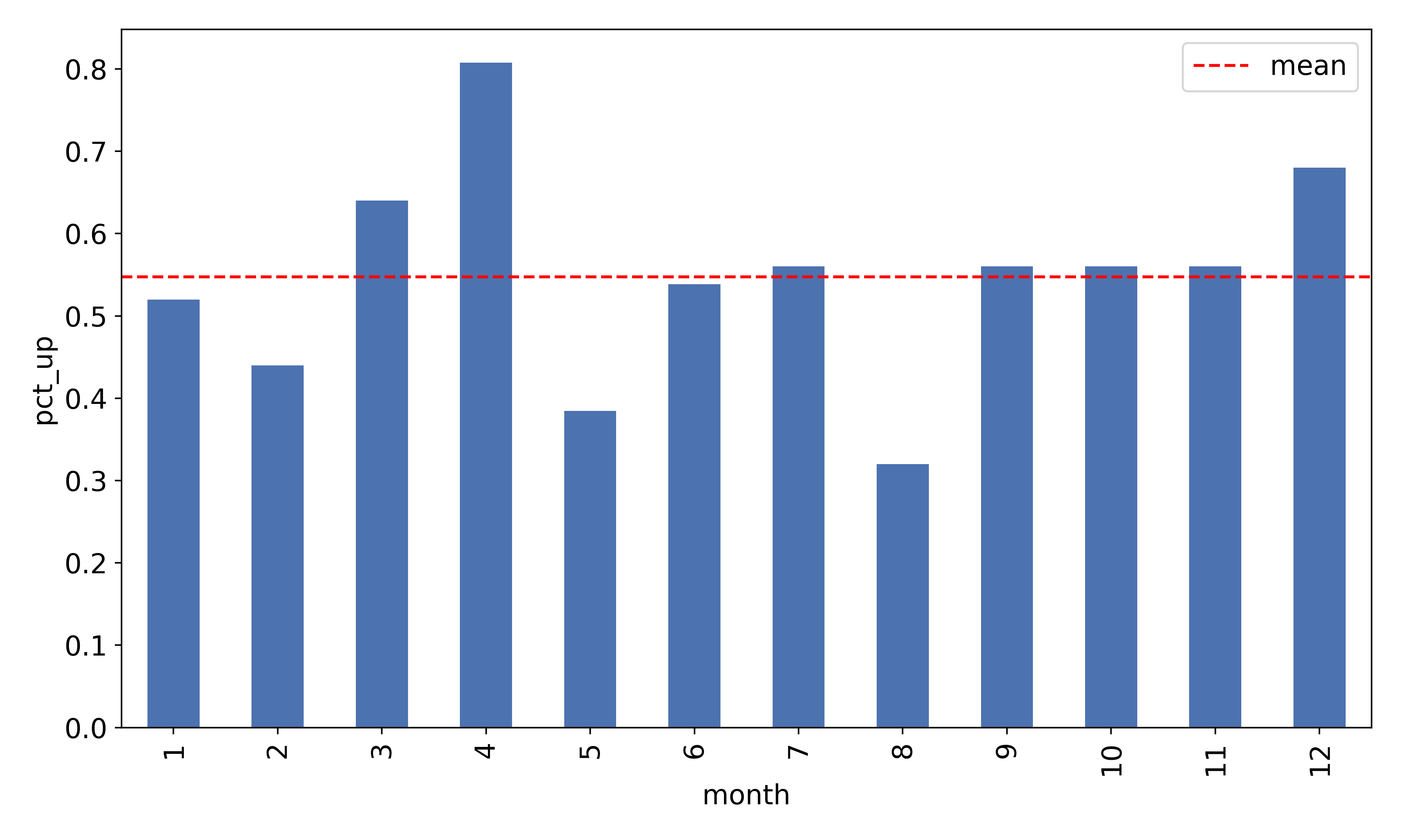
81% of April months showed positive returns. There is a discrepancy with respect to Mitchell’s results of 89%, likely because I used more data and a slightly different methodology for calculating returns. However, I think it is fair to say that we have replicated the anomaly.

With this in mind, a suitable null hypothesis might be “there is no seasonality in EWS returns”. To estimate a p-value, we need to generate many alternate EWS price series assuming there is no seasonality, then count the number of runs in which we nevertheless see an 81% seasonality. It is worth taking a moment here to convince yourself that this procedure does indeed give you the p-value.

The hard part here is simulating new EWS price series under the null hypothesis that there is no seasonality. How can we do this without assuming a distribution of returns? How can we create alternative realities in which everything is the same about EWS, except that it has no seasonality?

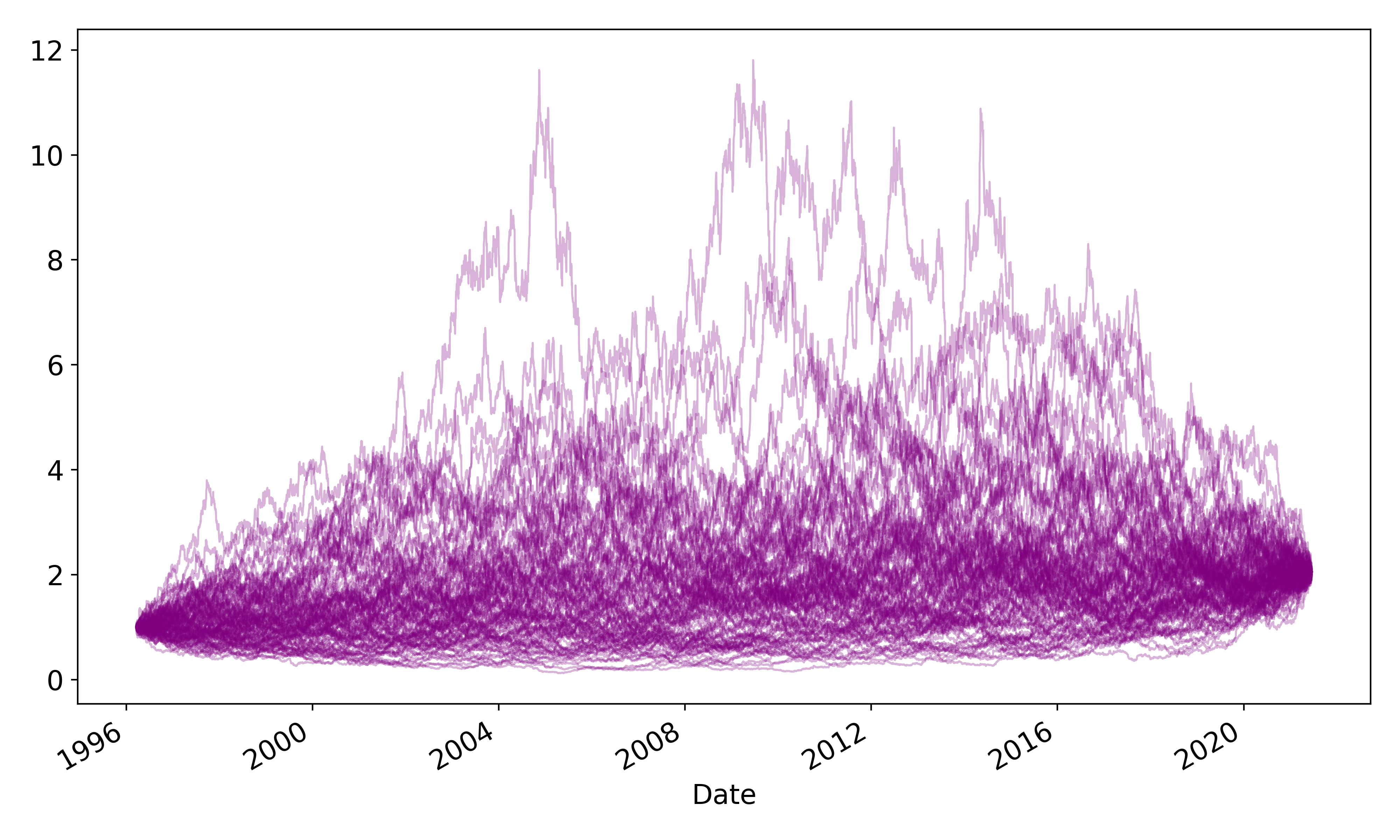
Here’s one solution: for each Monte Carlo run, construct a price series from the shuffled daily returns of the EWS time series. This generates alternative paths of EWS with the same mean and volatility as the original EWS time series (since these formulae are invariant under reorderings), but by shuffling, we are ensuring that there is no seasonality in the data-generating process.

def generate_path(rets):
    # rets is the daily EWS returns
    ret_shuffled = rets.sample(frac=1)
    ret_shuffled.index = rets.index
    px_new = (1 + ret_shuffled).cumprod()
    return px_new

Note that this doesn’t mean that any given Monte Carlo run will lack seasonality – the whole point of this exercise is to see how often a path will show seasonality given that there is no actual seasonality (i.e assuming the null hypothesis is true).

I generated 10,000 paths by reshuffling returns. For each path, I stored the maximum seasonal return (i.e for each month, calculate the percentage of months which had positive returns, then take the maximum percentage).

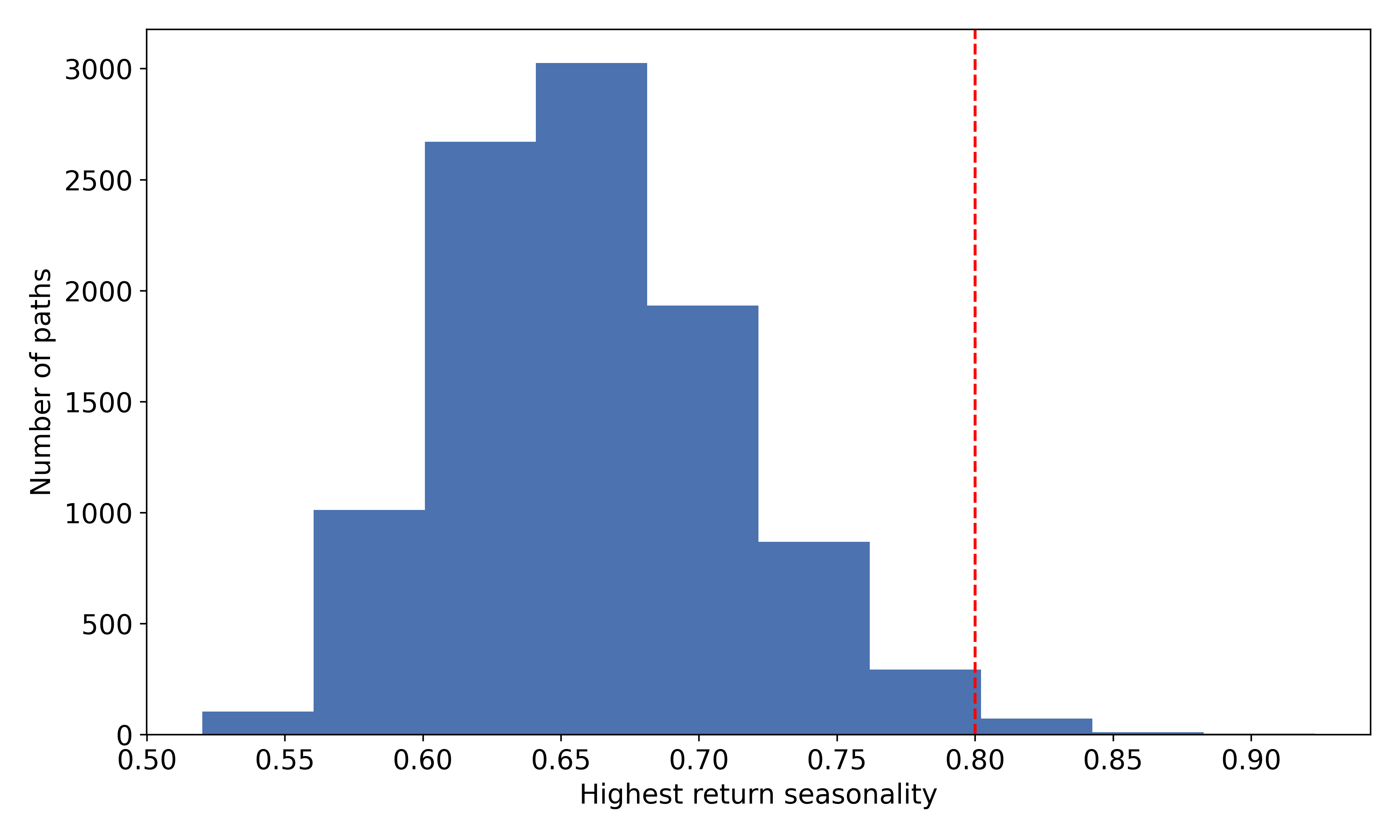
It turns out that only 72 out of the 10,000 paths had seasonalities as high as 80% (remember that we observed 81% in real life).

We therefore see that the p-value – the probability that we observe 80% seasonality purely by random chance (no actual seasonality) – is approximately equal to 0.7%.

Using the standard 5% significance level, we reject the null hypothesis and conclude that this anomaly is statistically significant.

Advice on setting up experiments

There is a slight art in figuring out how to set up these Monte Carlo hypothesis tests – it may not be immediately obvious how to generate data assuming the null hypothesis is true.

The question you need to answer is as follows: how can I randomly generate many paths of the time series with the same statistical properties as your observed data, except removing one particular property (whichever property you’re testing).

For anything to related to autocorrelations or seasonal effects, shuffling the data is appropriate because it removes any phenomena related to ordering, while preserving the moments of the distribution.

Testing regime shifts is simple – you just resample from the “old” distribution and see if it can explain the properties of the “new” distribution. For example, if you want to test whether post-GFC volatilities are different to pre-GFC volatilities, generating data under the null hypothesis is as easy as resampling from the pre-crisis return distribution, computing volatilities, and seeing how many paths generate have volatilities as high as the observed post-GFC volatility.

Conclusion

The key takeway from this post is that we only have access to one run of history. It is immensely difficult to figure out which events/anomalies are idiosyncratic to this run of history, vs “true” anomalies that exist in the actual data-generating process.

Distinguishing between the statistical artefacts and true anomalies is critically important because the former cannot be relied upon to reoccur in the future, so any strategy designed to capture them will look fantastic in backtests but fail in live trading (unfortunately a common occurrence in algo trading).

To summarise: embrace counterfactuals. Figure out as much as you can about alternative realities if you want to have a better idea of how you’re going to fare in this one.