Option-implied probability distributions, part 2
In Part 1 of this series, we demonstrated that the prices of option butterfly spreads imply a probability distribution of prices for the underlying asset. In this post, we will first examine the limiting case of butterfly spreads. Then, we will tackle the industry-standard approach for constructing PDFs from option prices: interpolating in volatility space to generate a volatility surface, converting this into a continuous set of option prices, then applying the Breeden-Litzenberger formula to find the PDF.
This post will be slightly more technical than Part 1, but as before, I endeavour to explain the motivation behind the maths.
The supporting code for this post can be found in this Jupyter notebook.
The limiting case of narrow butterflies
As mentioned in the conclusion to Part 1, deriving the PDF from butterfly prices is not a perfectly accurate method, even assuming we had perfect pricing data with negligible bid-ask spreads. This is because we made the approximation that the payoff of a butterfly is binary: either the maximum payoff $\Delta K$ if the expiration stock price is on the central strike, or zero otherwise. This payoff, of course, is not binary as it contains a sloped portion.
However, the approximation gets better and better as we use narrower butterflies because the sloped portion becomes less significant. For example, to calculate the probability that the expiry price of the stock is \$340, it would be better to use the 339/340/341 butterfly (as we did in the previous post) than to use the 335/340/345 butterfly, even though both of them are valid butterflies centred on \$340. Unfortunately, in the real world, we are not able to construct arbitrarily narrow butterflies because there is a limit to the granularity of strike prices on exchanges (with a \$1 granularity being typical for retail brokerages).
Let’s pretend we could construct arbitrarily narrow spreads. We will now show that in this limit $\Delta K \to 0$, the butterfly-implied probability converges to the PDF. The argument is rather mathematical and can be skipped, but do take a moment to appreciate the result. I find this little fact to be extremely exciting because it’s a clear case in which an initial intuitive approach (inferring the probability from the prices of butterfly spreads) actually converges to the right answer.
Recall that for a butterfly with price X and maximum payoff $\Delta K$, the probability $p_K$ that the underlying is at the central strike K at expiry (in which case the maximum payoff $\Delta K$ is received) can be found by an expected value calculation:
\[p \Delta K = X \implies p = \frac{X}{\Delta K}\]Probability density is not the same as probability; the general intuition is that probability is given by the area under a PDF – in fact, we can define the PDF as the function $f(x)$ such that:
\[P(A \leq x \leq B) = \int_A^B f(x)dx.\]With this in mind, the probability that the underlying price is within a small band $\Delta K$ of a given strike $K_0$ at expiry is:
\[P(K_0 \leq K \leq K_0 + \Delta K) \approx f(K_0)\Delta k.\]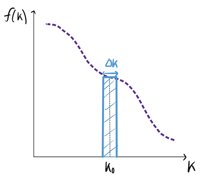
The approximation becomes an equality in the limit of small $\Delta K$. Hence, denoting $P(K_0 \leq K \leq K_0 + \Delta K)$ as $p_K$, we have:
\[p_K = \lim_{\Delta K \to 0} \left\{f(K)\Delta K \right\} \implies f(K) = \lim_{\Delta K \to 0} \frac{p_K}{\Delta K}.\]But we have an expression for $p_K$ in terms of the price, and can express the price of the butterfly in terms of the prices of the underlying call options (two short calls with strike $K$; long calls at strikes $K \pm \Delta K$):
\[\begin{aligned} f(K) &= \lim_{\Delta K \to 0} \left\{\frac{X / \Delta K}{\Delta K} \right\} = \lim_{\Delta K \to 0} \left\{ \frac{X}{(\Delta K) ^2} \right\} \\ &= \lim_{\Delta K \to 0} \left\{ \frac{C(K + \Delta K) - C(K) - C(K) + C(K- \Delta K))}{(\Delta K) ^2} \right\} \end{aligned}\]The astute reader will note that the RHS of this expression has a very familiar structure – it is the second (partial) derivative of the call price with respect to the strike price. The PDF can thus be expressed as:
\[f(K) = \frac{\partial^2 C(K)}{\partial K^2}\]This is an incredibly powerful result that relates the PDF directly to the prices of call options; furthermore, it shows that the limit of narrow butterfly spreads does indeed give the correct answer.
An alternative derivation
For those of you who are not intellectually satisfied by the intuitive derivation above, there is a slightly more rigorous argument (equally elegant, in my view).
By definition of the PDF, $P(S_T > K) = \int_K^\infty f(x)dx$ (here we are using x as a dummy variable for the strikes). As discussed in Part 1, the fair value of a call option (with time $\tau$ until expiry) is the present value of the expected payoff:
\[\begin{aligned} C(K, \tau) &= e^{-r\tau} \mathbb{E}(\max[S_T-K, 0]) \\ &= e^{-r\tau} \int_0^\infty \max[S_T-K, 0] f(S_T) dS_T \\ &= e^{-r\tau} \int_K^\infty (x-K)f(x)dx \end{aligned}\]The goal is to invert this to find $f(x)$ as a function of C. This can be done by expanding the integral and taking partial derivatives with respect to strike.
\[\begin{aligned} C(K, \tau) &= e^{-r\tau} \left[ \int_K^\infty xf(x)dx - K\int_K^\infty f(x)dx\right] \\ \implies \frac{\partial C}{\partial K} &= -e^{-r \tau} \int_K^\infty f(x)dx \\ &= e^{-r \tau} \left[ \int_{-\infty}^K f(x)dx -1 \right] \end{aligned}\]We now observe that $\int_{-\infty}^K f(x)dx$ is the definition of the cumulative distribution function $F(x)$, the derivative of which gives the PDF. Hence:
\[\frac{\partial^2 C}{\partial K^2} = e^{-r\tau} \frac{d}{dk} F(K) \implies f(K) = e^{r\tau} \frac{\partial^2 C}{\partial K^2}\]We have now derived the same result as before, generalised to include the time to expiry. The proper name for this result is the Breeden-Litzenberger formula (derived in their 1978 paper), a very useful tool which can convert call option prices into an implied PDF.
A detour into volatility space
Unfortunately, we cannot immediately apply the Breeden-Litzenberger formula to call prices for the same reason that butterfly spreads can’t be made arbitrarily narrow: strike prices come in discrete increments. To numerically calculate the second derivative of the call price function with respect to strike, we need our call prices to be near-continuous with respect to the strike, requiring interpolation (possibly some signal smoothing first).
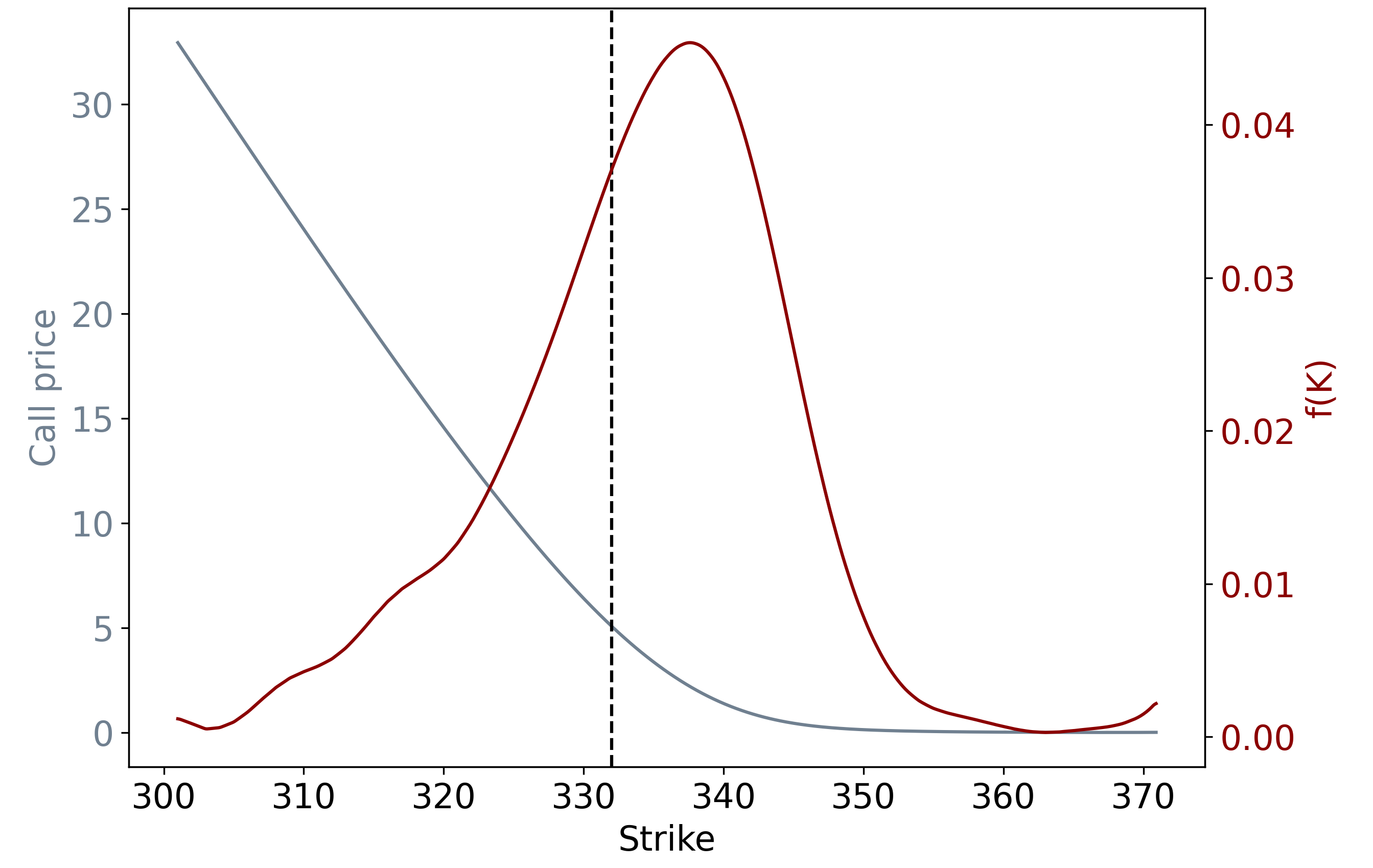
At this juncture, two roads diverge in a yellow wood. The obvious thing to do is to interpolate in price-space, i.e join the dots in the below plot:
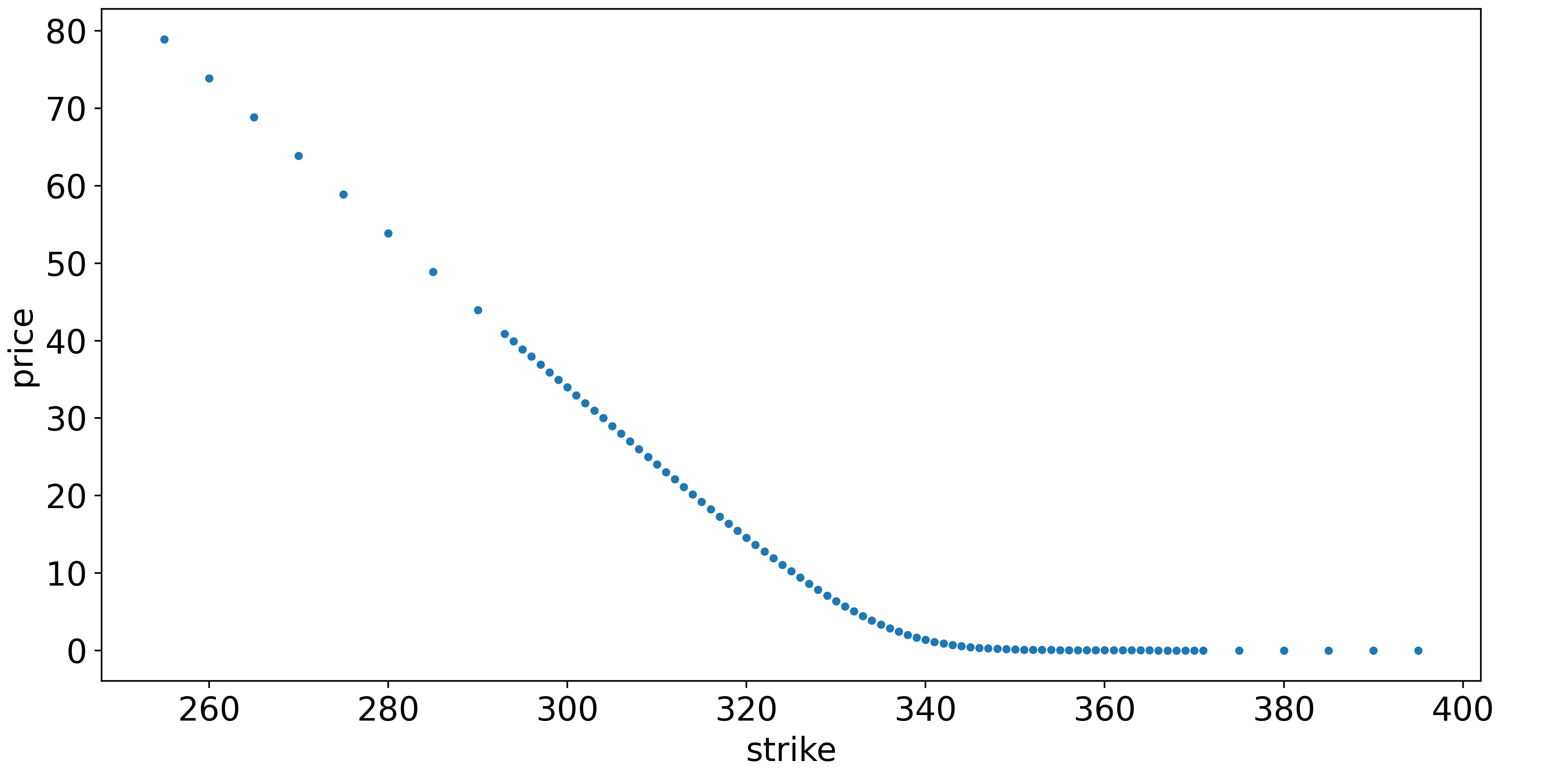
This seems straightforward, but there is a catch. It is dangerously easy for interpolation to result in arbitrage opportunities (which are not realistic). For example, any straight-line interpolation, such as setting the price of the \$105-strike option to be exactly between the prices of the \$100- and \$110-strike options, leads to a free butterfly spread. In fact, with the Breeden-Litzenberger formula in mind, any interpolation must always be convex (positive second derivative with respect to strike) since the PDF must be positive. If you are a market maker, mispricing the options to allow for arbitrage opportunities would be a cardinal sin, because you would make a guaranteed loss while your counterparty makes a risk-free profit.
It is essential, therefore, to be cautious when interpolating. One reason for the instability of interpolation in “price space” is that the price can be thought of as the dependent variable (i.e output) of an option pricing model which has several inputs:
- The price of the underlying and the strike (further OTM is less valuable)
- Time to expiration (more time is more valuable)
- Volatility (more volatile is more valuable)
- Interest rates (higher rates means calls are more valuable)
- Dividends (higher dividends means calls are less valuable)
(The last two are much less important than the first three). The argument goes that it makes more sense to interpolate on the inputs to this function versus the output (price) because inputs should be “smoother” than outputs. The moneyness of the option and the time to expiration are pre-determined when entering a contract, so the only meaningful free input parameter which we might consider interpolating is the volatility.
Black-Scholes and implied volatility
I can’t avoid bringing up Black-Scholes, but this is certainly not the place to give a detailed introduction to the theory.
The Black-Scholes model values an option – it does not price an option any more than a discounted cash flow analysis prices a stock – by making several assumptions: the volatility of the underlying is constant, the returns of the underlying are normally distributed, efficient markets, etc. As anyone who has witnessed Nassim Taleb’s Twitter vitriol will know, these assumptions are often far from the truth.
Instead of proceeding with this definition, for the purposes of this post, let’s forget everything we know about Black-Scholes and redefine it as follows:
- There is a function called
Black-Scholeswhich converts implied volatilities (IVs) – to be defined – into option prices. - There is a function called
Black-Scholes Inversewhich converts option prices into IVs.
That’s it. Nothing about pricing or valuing options. No assumptions about the distribution of asset returns. Just a mathematical identity.
The reason we can get away with this bold claim is that there is an embedded circularity. “Implied volatility” is defined to be the volatility which results in the current option price when input to standard Black-Scholes. It might seem like we have just done some Lewis Carroll-esque wordplay, but for reasons we shall soon see, this circularity can be much more workable than the alternative of trying to define IV along the lines of the “expected future volatility”.
In summary, price and IV can be interchanged by applying the appropriate function. This allows us to make the key insight: rather than interpolating in price space, we can convert the prices to IVs using Black-Scholes Inverse, interpolate in IV space, then convert the interpolated IVs back to prices using Black-Scholes.
Interpolating in IV space
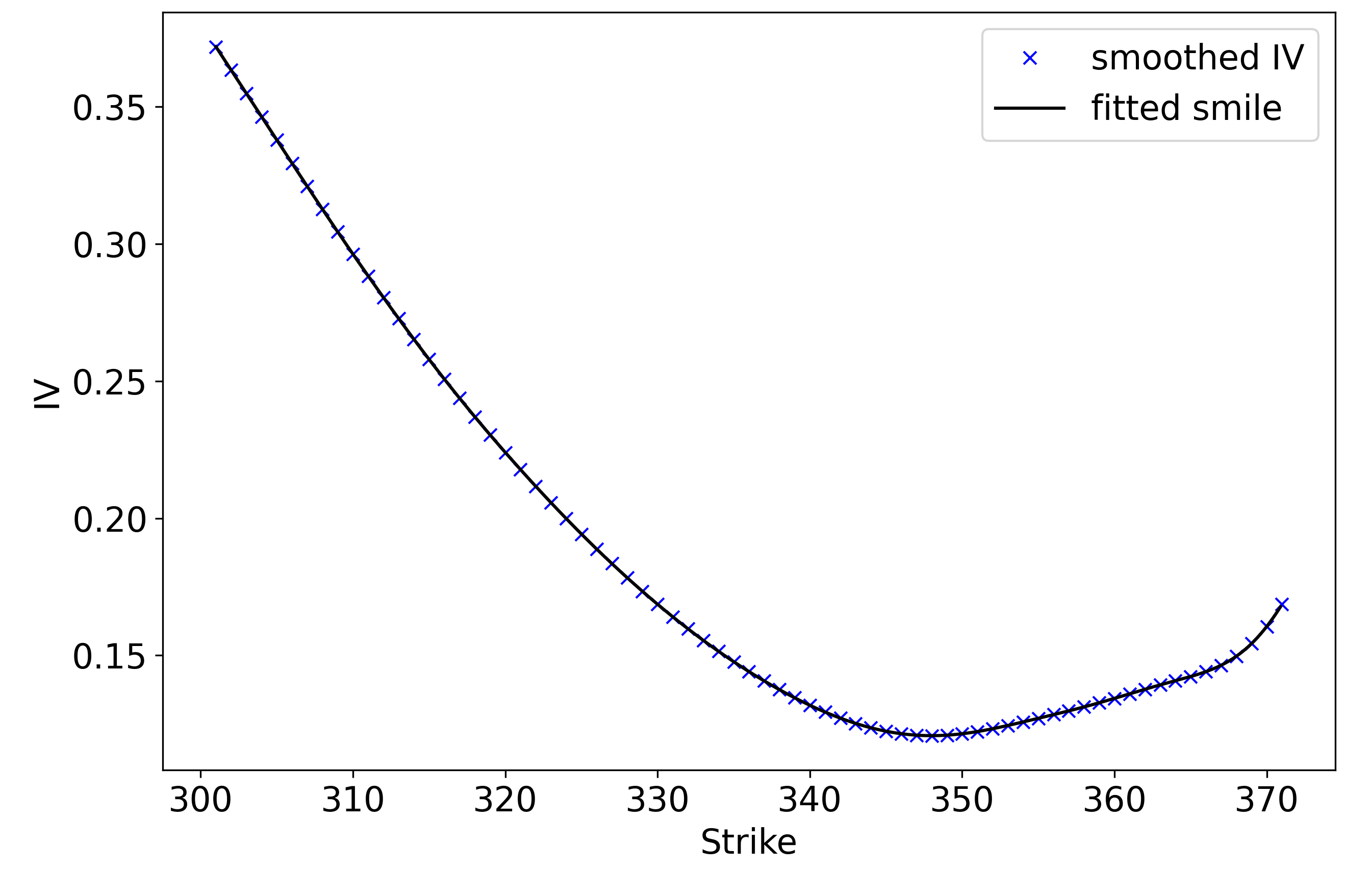
Using the same SPY dataset as in Part 1 (collected when $S = \$332$ with about 3 weeks to expiry), the first step is to use Black-Scholes Inverse to bring us from price space into IV space.
There is no closed-form inverse to the Black-Scholes formula, so Black-Scholes Inverse is a numerical method – I chose to use Newton’s method, because it is easy to code up, but be aware that even the topic of computing IVs has been deeply researched. Excluding some pathological deep ITM/OTM contracts, the result of Black-Scholes Inverse is shown below:
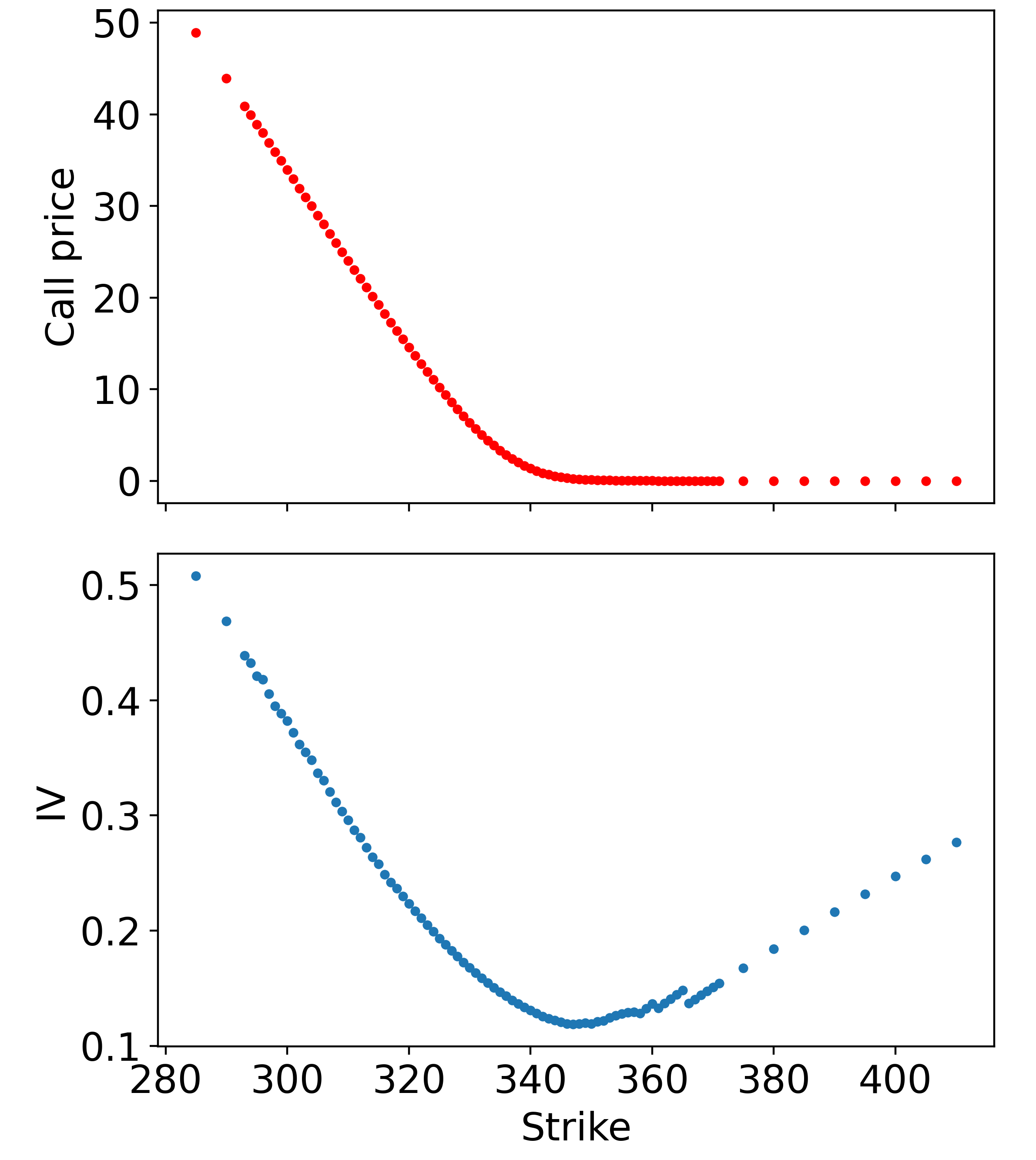
There are some problems around the \$365-strike contracts, but after applying a Gaussian filter and clipping out additional deep ITM/OTM contracts, we have something workable:
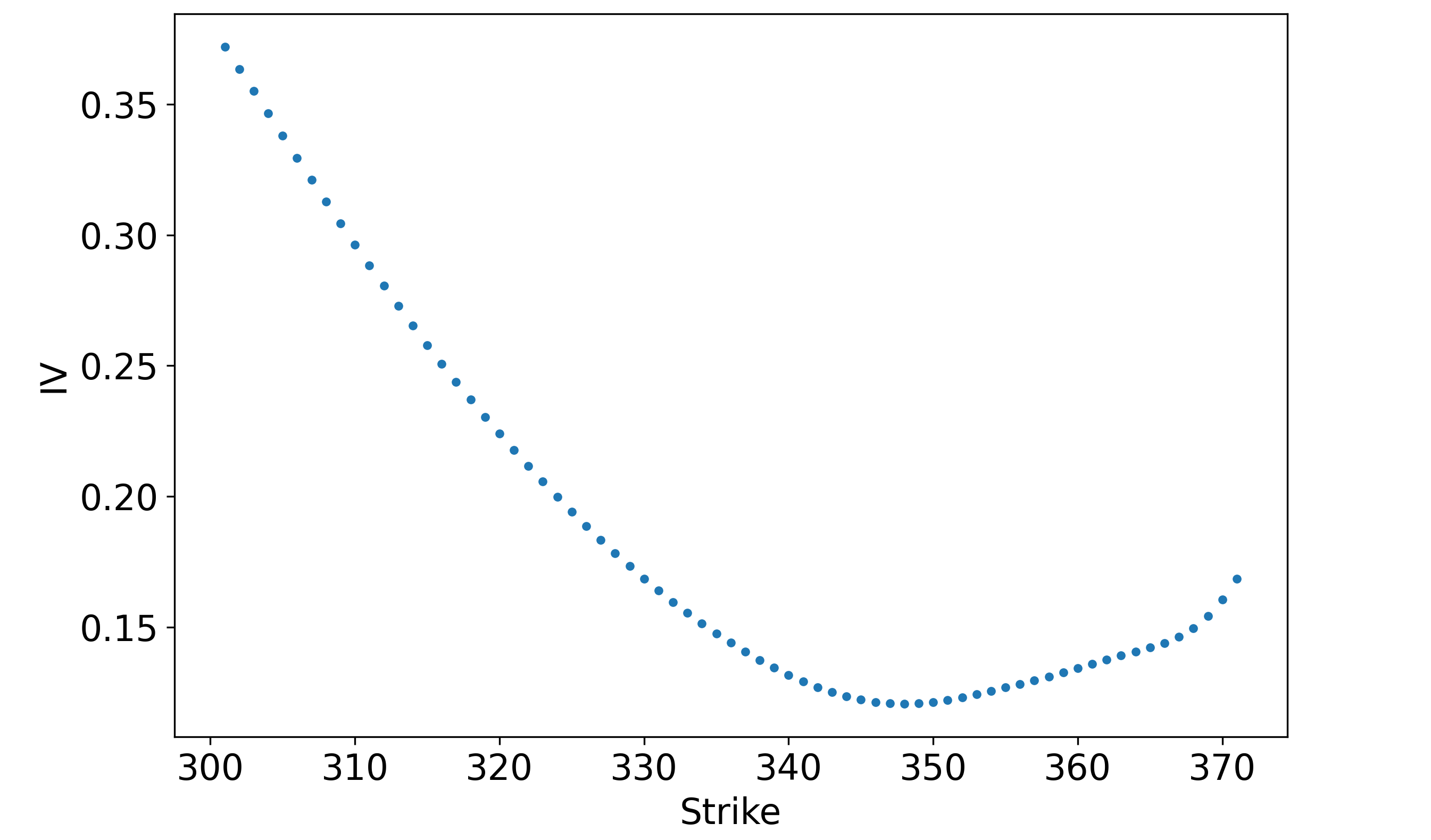
We can then apply the same cubic spline that we used with the butterfly probabilities to create a smooth function – a cross-section of the volatility surface.
With a moment’s reflection, this plot is rather unintuitive. Rather than having a constant IV, we observe the characteristic volatility smile. This does not make much sense if we think of IV as the “expected wiggliness” of returns in the underling between now and expiry – the future volatility should be independent of the strike – and is in clear contradiction to the Black-Scholes assumption that volatility is constant.
Instead, using the “circular” definition that IV is the input volatility to Black-Scholes that results in the observed call price, we can rationalise the volatility smile as follows: buyers are willing to pay a premium (relative to the Black-Scholes “fair value”) for out-of-the-money options. A classic explanation for this is that asset returns typically have fat tails, meaning that OTM options are more valuable than Black-Scholes would suggest.
Constructing the PDF of underling prices
Having interpolated in volatility space, we can convert back to price space using Black-Scholes, then take the second partial derivative of the call function with respect to strike (numerically) to find the PDF, as per the Breeden-Litzenberger formula:
Comparing PDFs
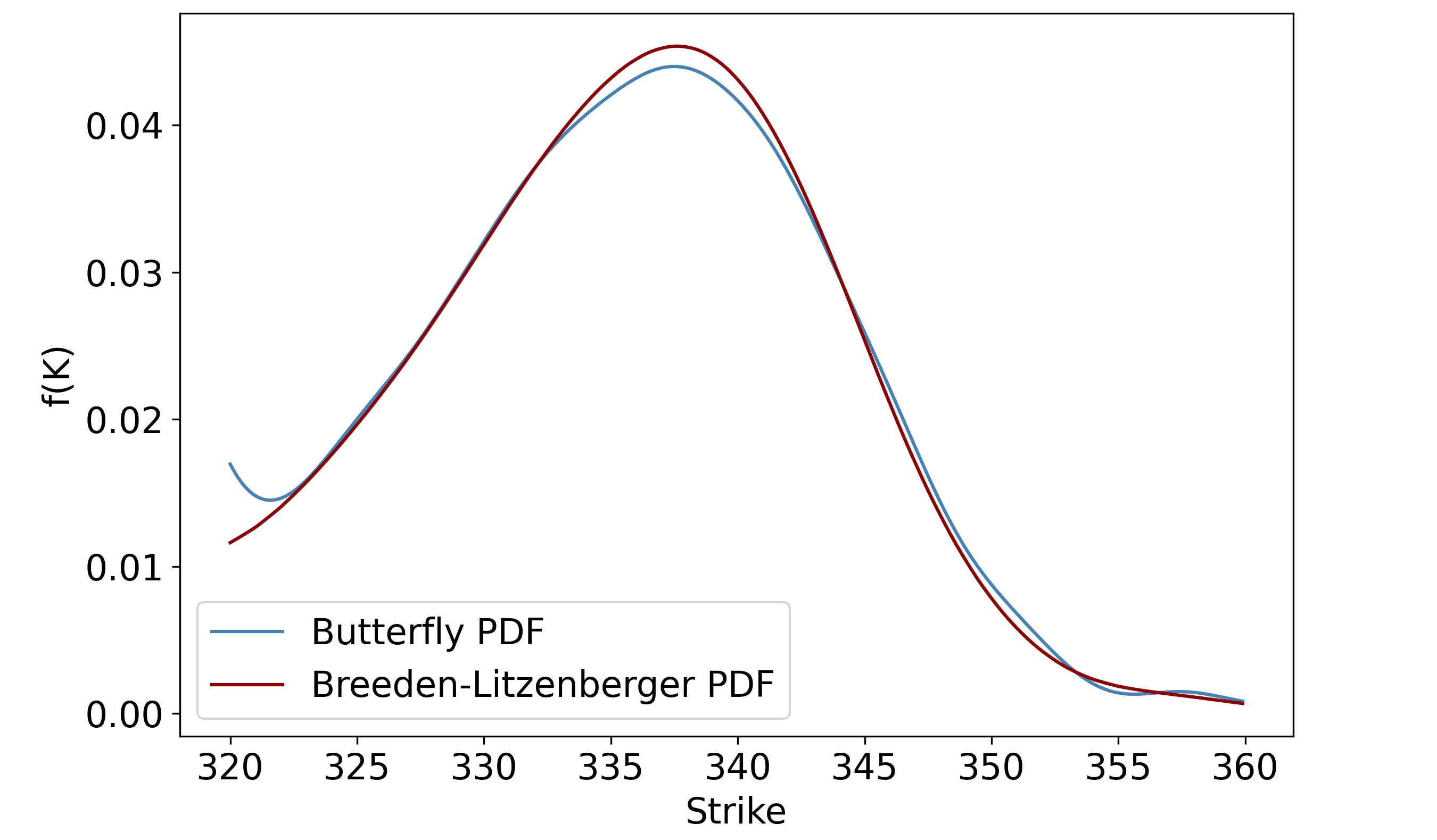
We can now compare the butterfly PDF that we generated in the previous post with the Breeden-Litzenberger PDF. Firstly, as seen above, the Breeden-Litzenberger method gives us a larger range of strikes (\$300-\$370 vs \$320-\$360 for butterfly PDFs), which makes sense because constructing each butterfly requires three price quotes.
Secondly, even after restricting the range of strikes to be the same as for the butterfly PDF, note that the Breeden-Litzenberger PDF is better-behaved, lacking the kinks at $355 < K < 360$ (though as the previous plot shows, it does start to wobble as we move away from at-the-money):
The last thing we ought to do is compare the two roads that diverged in the yellow wood: interpolation in IV space vs interpolation in price space – recall that these are two methods of generating a continuous call function, after which Breeden-Litzenberger can be applied.
Using the same Gaussian filter and cubic spline, we can smooth and interpolate the call prices directly. The resulting PDFs is compared with the IV-space interpolation PDF below:
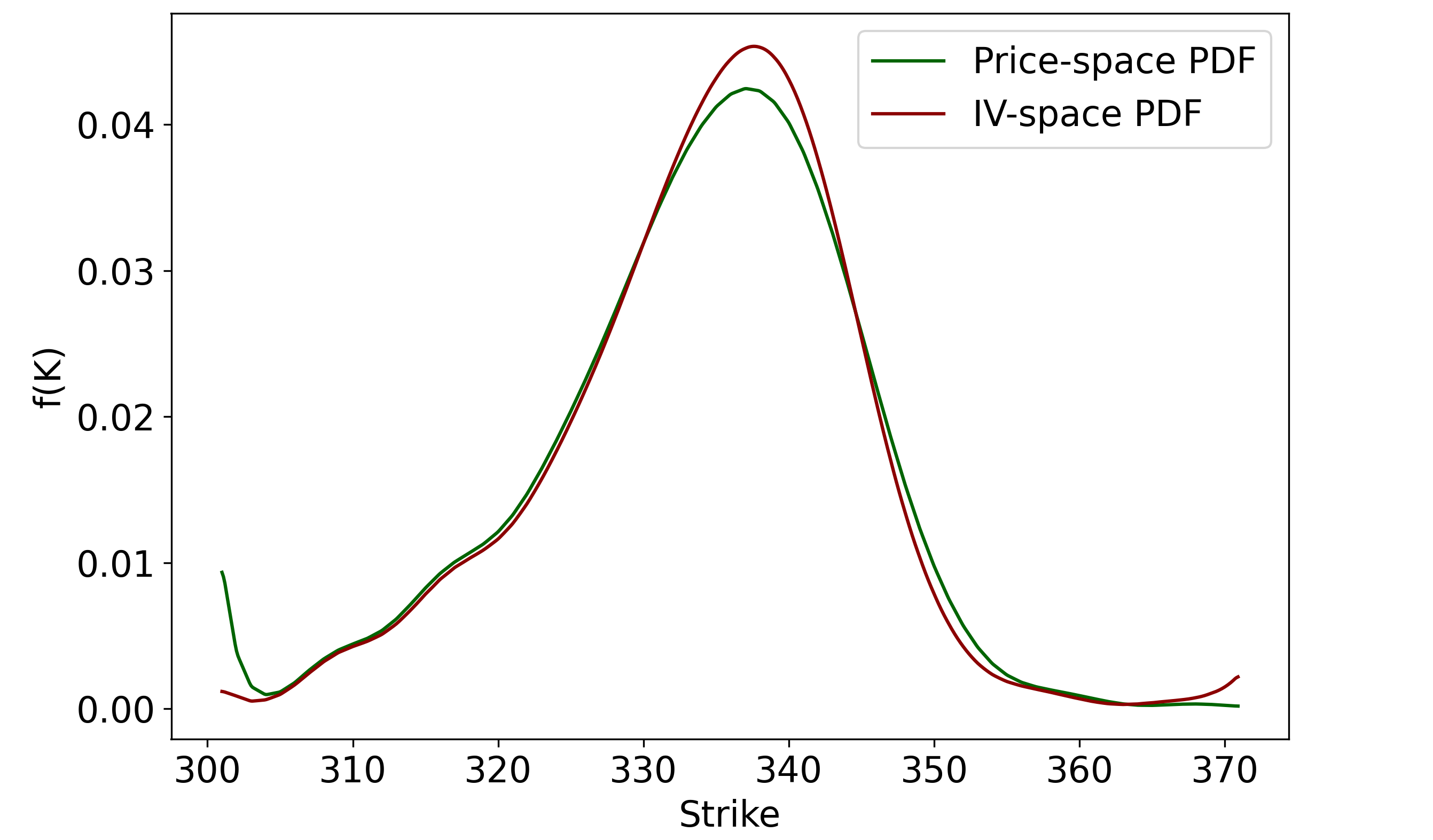
The IV-space approach seems to give much better results in the left tail, but slightly worse results in the right tail. Overall, there does not appear to be strong evidence that interpolating in IV-space is superior to interpolating in price-space, at least for this particular example, but I do think that interpolating in IV-space is logically more defensible.
Conclusion
In conclusion, this pair of posts has given an introductory overview of how we might construct price PDFs by looking at option prices.
There is much more that could be said about this subject. For example, we have completely ignored half of the available data – the prices of put options. A common technique is to use put-call parity to generate more data points for fair prices of call options, improving our estimate of the volatility surface. Furthermore, this post has taken a non-parametric approach, i.e we have not assumed that the volatility smile has any shape. In practice, parametric models are popular because they lead to smooth and analytically tractable surfaces.
I realise that I have not spent a great deal of time explaining why we might want the option-implied PDF. The obvious answer is that if you know the option-implied PDF, you can understand the market’s probabilistic expectations of the future and make trades when your view differs. What is not obvious is how one might generate probabilistic views in the first place. This is a topic that I will be revisiting in a subsequent post – this series was written solely to lay the groundwork for an upcoming piece, in which I am hoping to approach fundamental valuation from a probabilistic perspective.