Algorithms

These algorithms are coded in a python-like pseudocode, but in some cases the pseudocode is actually valid python!

Complexity
Sorting Algorithms
Dynamic programming
Greedy algorithms
Other solution strategies
Graph algorithms
Geometrical algorithms
- Graham’s scan

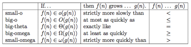
Complexity

\[f(n) \in O(g(n)) \Longleftrightarrow \exists N, c_1, c_2 >0 \text{ s.t. } \forall n > N: 0 \leq g(n) \leq k g(n)\]

More informally, we can define other asymptotic notation as follows:

In the analysis of algorithms, many assumptions about hardware and basic operations must be made, e.g. array access is constant time.

Sorting Algorithms

Sorting is important because we can use binary search on sorted arrays in $O(\log n)$ time.
In the worst case, $\Theta(n)$ exchanges will be needed.
Comparison-based algorithms require at least $\Omega(n\lg n)$ comparisons.

Insertion Sort

Maintain a sorted section of the array, then insert new items into the correct position.

def insertion_sort(a):
    for i in range(1, len(a)):
        # assert first i positions sorted
        j = i - 1
        while j >= 0 and a[j] > a[j+1]:
            swap(j, j+1)
            j -= 1  

Inserting the last element needs at most $n-1$ comparisons and swaps. The second last element requires $n-2$…

\[T(n) = 2 (1 + 2 + \cdots + n - 1) = n(n-1)\]

So insertion sort is $O(n^2)$. That said, it has a very small constant term so is often faster than $O(n \lg n)$ algorithms for small n.
It is stable as long as we only swap if the element is larger than the key.

Selection sort

At each iteration, find the minimum of the remaining array and swap it to the current index.

def selection_sort(a):
    for i in range(len(a)):
        swap(i, argmin(a[i:end]))

$O(n^2)$ and unstable. Its only advantage is that it is easy to analyse.

Binary insertion sort

Same as insertion sort, except we find the correct position using binary partitioning.

def binary_insertion_sort(a):
    for i in range(1, len(a)):
        hi = i
        lo = 0
        while lo < hi:
            j = (hi + lo) // 2
            if a[i] > a[j]:
                lo = j + 1
            else:
                hi = j
        
        # Swap a[i] into the right place
        tmp = a[i]
        for j from i - 1 down to (hi - 1):
            a[j+1] = a[j]
        a[hi] = tmp

Binary insertion sort will be preferred to insertion sort when comparisons are expensive, but the swapping costs mean that it is still $O(n^2)$.

Bubblesort

In each pass, go through the list swapping adjacent elements as needed. If no swaps are done in a pass, the array is sorted.

def bubblesort(a):
    while True:
        didSwap = False
        for i in range(len(a) - 1):
            if a[i] > a[i+1]:
                swap(i, i+1)
                didSwap = True
        if not didSwap:
            break

In the worst case, an element will be n positions away from its final position, so the complexity is $O(n^2)$.
Stable

Mergesort

Divide and conquer algorithm that splits the list in two then recursively sorts each half, before merging sorted lists.

def mergesort(a, lo, hi):
    if lo < hi:
        mid = (lo + hi) // 2
        mergesort(a, lo, mid)
        mergesort(a, mid+1, hi)
        merge(a, lo, mid, hi)
        
def merge(a, lo, mid, hi):
    # both these subarrays are sorted
    l = a[lo: mid]
    r = a[mid+1 : hi]
    
    aux = [] * (len(l) + len(r))
    
    i = lo
    j = mid + 1
    
    for k in range(len(aux)):
        if i > mid: # fill using right only 
            aux[k] = aux[j]
            j += 1
        else if j > hi: # fill using left only
            aux[k] = a[i]
            i += 1
        else if a[i] <= a[j]: # otherwise compare
            aux[k] = a[i]
            i += 1
        else:
            aux[k] = a[j]
            j += 1

$\Theta (n \lg n)$ runtime, but requires $O(n)$ extra space.
Mergesort is stable because there is no reordering of equal elements.
Mergesort can instead be implemented bottom-up, merging pairs, then pairs of pairs, then pairs of fours, etc.

def mergesort(a):
    step = 1
    while (step < len(a)):
        for lo in range(0, len(a), 2*step):
            mid = lo + step - 1;
            hi = min(lo + 2*step - 1, len(a) - 1);
            merge(aux, lo, mid, hi);    

Quicksort

Choose the last item as the pivot, then partition the array into items ≤ the pivot and items > pivot. Put the pivot in the middle then recursively sort left and right.

def quicksort(a):
    pivot = a[len(a) - 1]
    i = 0
    j = len(a) - 2
    
    while i <= j:
        if a[i] > pivot and a[j] <= pivot:
            swap(i, j)
            i += 1
            j -= 1
        else if a[i] <= pivot:
            i += 1
        else: j -= 1
        
    # ASSERT i == j + 1
    # ASSERT all items to the left of i <= pivot
    swap(j, len(a) - 1)
    quicksort(a[0:j])
    quicksort(a[j+1:end])

$O(n \lg n)$ average case, $O(n^2)$ worst case.
Requires $O(\lg n)$ additional space to store stack frames, but $O(n)$ in the worst case.
Unstable.

Order statistics

A quicksort-like algorithm can be used to compute the median and, more generally, order statistics.

Select a pivot and partition the array into subarrays of size $p$ and $n-p$
If $k < p$, recursively look for the kth item in the lower partition.
Otherwise recurse into the upper partition to find rank $k-p$

This has recurrence:

\[T(n) = f(n/2) + kn = O(n)\]

However, the worst case is $O(n^2)$ as with quicksort. There exists a guaranteed linear time algorithm but it is much more complicated.

Heapsort

Turn the array into a max-heap in $O(n)$
Swap last item with max, reduce heapsize, then heapify down.
Repeat until heapsize is 0.

def heapsort(a):
    for i in range(len(a) // 2, 0 included):
        heapify(a[i], i, len(a))
            
    for k in range(len(a), 1):
        # a[0:k] is a max-heap
        # a[k:end] is sorted
        swap(0, k - 1)
        heapify(a, 0, k-1)
        
def heapify(a, iRoot, iEnd):
    if a[iRoot] satisfies max-heap:
        return
    
    j = largest child of iRoot
    swap(iRoot, j)
    heapify(a, j, iEnd)

Runtime $O(n \lg n)$

Counting sort

Counting sort does not require comparisons. Assuming that the inputs are positive integers within some range, it counts the number of each element, then finds the cumulative sum, from which we can identify exactly where a given element should go.

def counting_sort(a):
    count = [0] * max(a)
    for x in a:
        count[x] += 1
    # cumulate
    for i in range(1, len(count)):
        count[i] += count[i-1]
    
    sorted = [0] * len(a)
    for i in range(len(a) - 1, 0 included):
        idx = count[a[i]] - 1
        sorted[idx] = a[i]
        count[a[i]] -= 1
    return sorted

It is a stable sorting algorithm, with $\Theta(n)$ cost.

Bucketsort

Bucketsort creates an array of buckets (linked lists), with the assumption that elements will fall into these buckets uniformly. We can then run insertion sort within each bucket before concatenating the buckets into a sorted array.

def bucket_sort(a):
    # assuming that elements are drawn uniformly from [0,1]
    n = len(a)
    bucketWidth = 1/n
    buckets = new [] of length n
    
    for x in a:
        idx = int(x / bucketWidth)
        bucket[idx].next = x
    
    sorted = []
    for b in buckets:
        insertion_sort(b)
        sorted.append(b)
    return b

We use insertion sort because each bucket should contain only one element on average. But the worst case is still $O(n^2)$ as a result.

Radix sort

Assuming all elements have the same number of digits, we use a stable sort each column starting from the least significant digit.

def radix_sort(a, d):
    for i in range(1, d):
        stable_sort(a on digit i)

$O(n)$ if counting sort is used for digits.

Dynamic programming

Dynamic programming tends to be useful when problems have the following features:

There exist many choices each with some ‘score’
The optimal solution is composed of optimal solutions to subproblems
The subproblems overlap.

Memoization is a technique often used in top-down dynamic programming:

Memoization is a time-space trade-off which in which results to computations are stored (in an array or hashtable) so we don’t have to recompute results.
The table will be persistent between function calls, and every invocation will check whether its arguments correspond to a previously-computed result. If so, we can return it in constant time.

Greedy algorithms

At every stage, choose the ‘current best action’ without considering the values of the actions in subsequent states.
It is necessary to prove that the greedy choice plus an optimal solution to the subproblem leads to an overall optimum solution.
Most greedy problems can be solved as DP problems but the greedy approach is more efficient (when valid).

Graph algorithms

DFS

Used to traverse or search a graph.

def dfs(g, s):
    for v in g.vertices:
        v.visited = False
    s.visited = True

    stack = Stack()
    stack.push(s)
    
    while not stack.empty():
        v = stack.pop()
        for w in v.neighbours:
            if not w.visited:
                stack.push(w)
            w.visited = True

$O(V+E)$ runtime

BFS

Used to traverse or search a graph.

def bfs(g, s):
    for v in g.vertices:
        v.visited = False
    s.visited = True

    q = new Queue()
    q.push(s)
    
    while not q.empty():
        v = q.pop()
        for w in v.neighbours():
            if not w.visited:
                q.push(w)
            w.visited = True

To use DFS or BFS to find a path, we just have to update a previous field for each node, then walk back from the target to the start.
$O(V+E)$ runtime

Dijkstra

After running Dijkstra, the distance field contains the minimum distance from s to that vertex.
Similar to BFS, except we use a priority queue to store vertices. If we visit a vertex that has already been seen, we update its distance and its position in the priority queue.

def dijkstra(g, s):
    for v in g.vertices:
        v.distance = infinity
    s.distance = 0
    
    pq = PriorityQueue(sortkey = lambda v: v.distance)
    pq.push(s)
    
    while not pq.empty():
        v = pq.popmin()
        for (w, edgecost) in v.neighbours:
            dist = v.distance + edgecost
            if dist < w.distance:
                w.distance = dist
                
                if w in pq:
                    pq.decreasekey(w)
                else: 
                    pq.push(w) 

$O(E + V \log V)$ runtime

Bellman equation

Used to find minweight path (i.e same as Dijkstra but works for negative weights)
$W_{ij}$ is the minweight action to go from state i to j:

\[W_{ij} = \begin{cases} 0, & i = j\\ \text{weight}(i \to j), & \text{if there is an edge} \\ \infty, & \text{otherwise} \\ \end{cases}\]

The minimal weight path from i to j in l steps is denoted by $M_{ij}^{(l)}$. We can compute it with dynamic programming.

\[\begin{aligned} M_{ij}^{(1)} &= W_{ij} \\ M_{ij}^{(l)} &= \min_k \{ W_{ik} + M_{kj}^{(l-1)}\} \end{aligned}\]

This can be formulated as a matrix multiplication, where $x \wedge y \equiv \min(x,y), n = |V|$.

\[M_{ij}^{(l)} = (W_{i1} + M_{1j}^{(l-1)}) \wedge (W_{i2} + M_{2j}^{(l-1)}) \wedge \cdots \wedge (W_{in} + M_{nj}^{(l-1)})\]

This is a brute force algorithm requiring $\log V$ matrix multiplications, so runtime is $O(V^3 \log V)$.

Bellman-Ford

Used to find the minweight path (i.e same as Dijkstra but works for negative weights)
Relax all the edges in a graph, for $V-1$ passes. If there are any changes in the last round, there is a negative weight cycle.

def bellman_ford(g, s):
    for v in g.vertices:
        v.minweight = infinity
    s.minweight = 0
    
    # relax all edges
    repeat len(g.vertices) - 1 times:
        for (u, v, c) in g.edges:
            if v.minweight > (u.minweight + c):
                v.minweight = u.minweight + c

    # check for negative cycles in last pass
    for (u, v, c) in v.edges:
        if v.minweight > u.minweight + c:
            raise NegativeWeightCycle()

$O(VE)$ runtime.

Johnson’s algorithm

Find the minimal weight paths between all pairs of vertices
Uses Bellman-Ford once to check for negative weight cycles, then makes weights positive and uses Dijkstra on every vertex.

def johnson(g):
    h = new Graph()
    h.add_vertex(s, weights=[0, 0, 0,...])
    
    bellman_ford(g, s)
    
    # Make edges positive
    for (u, v) in g.edges:
        w(u -> v) = h.u.distance + w(u -> v) - h.v.distance
    
    for v in g.vertices:
        dijkstra(g, v)

Runtime $O(VE + V^2 log V)$

Prim

Greedy algorithm to find a minimum spanning tree by choosing the lowest weight connector to a new vertex
Very similar to Dijkstra, except:
- need to keep track of the tree
- update distance from tree instead of distance from start
Returns the list of edges in the MST.

def prim(g, s):
    for v in g.vertices:
        v.distance = infinity
        v.in_tree = False
        
    s.come_from = None
    s.distance = 0
    s.in_tree = True
    
    pq = new PriorityQueue(sortkey = lambda v: v.distance)
    
    while not pq.empty():
        v = pq.popmin()
        v.in_tree = True 
        
        for (w, edgeweight) in v.neighbours:
            if edgeweight < w.distance and (not w.in_tree):
                w.distance = edgeweight
                w.come_from = v
                if w in pq:
                    pq.decreasekey()
                else:
                    pq.push(w)
    
    return [(w, w.come_from) for w in g.vertices excluding s]

Runtime the same as Dijkstra, i.e $O(E + V \log V)$.

Kruskal

Builds a minimum spanning tree by greedily merging subtrees, starting with V trees of order 0.

def kruskal(g):
    tree_edges = []
    partition = DisjointSet() 
    
    for v in g.vertices:
        partition.add_singleton(v)
        
    edges = sorted(g.edges, sortkey = edgeweight)
    
    for (u, v, edgeweight) in edges:
        p = partition.get_set_with(u)
        q = partition.get_set_with(v)
        
        if p != q:
            tree_edges.append((u, v))
            parition.merge(p, q)
            
    return tree_edges

Runtime is dominated by the sort: $O(E \log E) = O(E \log V)$.

Topological sort

Recursive DFS (for all nodes), prepend to list once visit(v) returns.

def topological_sort(g):
    for v in g.vertices:
        v.visited = False
        # v.colour = "white"
    
    totalorder = []

    for v in g.vertices:
        if not v.visited: 
            visit(v, totalorder)

    return totalorder
            
def visit(v, totalorder):
    v.visited = True
    # v.colour = "grey"
    for w in v.neighbours:
        if not w.visited:
            visit(w, totalorder)
    totalorder.prepend(v)
    # v.colour = "black"

Same runtime as DFS: $O(V+E)$

Ford-Fulkerson

Finds the maximal flow in a network (a graph where edges have positive capacities).
While possible:
- find an augmenting path in the residual graph by looking for spare capacity or removing it when there is an excess
- compute the bottleneck capacity of the augmenting path
- augment the flow in the original graph

def find_augmenting_path(g):
    # helper graph
    h = new Graph(g.vertices)
    
    for each pair of vertices (v,w) in g:
        if f(v -> w) < c(v -> w):
            h.add_forward_edge(v -> w)
        if f(w -> v) > 0: 
            h.add_backward_edge(v -> w)
        if h contains path(s to t):
            return path
        else:
            # no more paths
            return None

def ford_fulkerson(g, s, t):
    # zero flow initially
    for (u, v) in g.edges:
        f(u -> v) = 0
    
    while True:
        p = find_augmenting_path()
        
        if p is None:
            break

        delta = infinity # bottleneck
        for each edge (v1, v2) in p:
            if edge.forwards:
                delta = min(delta, c(v1 -> v2) - f(v1 -> v2))
            else:
                delta = min(delta, f(v2 -> v1))
                
        # Augment flow
        for each edge (v1, v2) in p:
            if edge.forwards: 
                f(v1 -> v2) += delta
            else:
                f(v2 -> v1) -= delta

Runtime is $O(Ef^*)$

Geometrical algorithms

Geometrical algorithms notes

Graham’s scan

Used to find the corner points on a convex hull.

def graham_scan(points):
    let r0 be the lowest point
    r = [r1, r2, r3, ..., rn]  = sort(points, sortkey=r.angle)
    
    S = new Stack([r1, r2, r3])
    for i in range(3, n):
        while r[i] is not on the left of the segment(S.first(), S.second()):
            S.pop()
        S.push(r[i])
    return S

Runtime is $O(n \log n)$ from sorting the points.

Reasonable Deviations