Conway's Game of Life in python
In this short post, I explain how to implement Conway’s Game of Life in python, using numpy arrays and matplotlib animations. I emphasise intuitive code than performance, so it could be a useful starting point for somebody to understand the logic before implementing a more efficient version.
Cellular automata
A cellular automaton (pl. automata) consists of a grid of cells; each cell has a state — either alive or dead. I will refer to this grid as the universe, though this is non-standard terminology. The automaton then iterates forward in time, with the new state of each cell being decided by a set of rules.
One of the most widely-studied cellular automata is the Game of Life, sometimes just called ‘Life’, which was discovered (or ‘invented’ if you prefer) by John Conway. It is so named because its rules can be interpreted as a very simplistic model of living cells.
Firstly, let us define the the eight grid squares around a cell as its neighbours. The rules of Life are then as follows:
1. A living cell will survive into the next generation by default, unless:
- it has fewer than two live neighbours (underpopulation).
- it has more than three live neighbours (overpopulation).
2. A dead cell will spring to life if it has exactly three live neighbours (reproduction).
Clearly, no cells can come to life unless there are already some living cells in the universe (Aquinas’ primum movens?). Thus, we have to provide the universe with a seed, i.e a set of initial living cells. The massive variety and complexity of the results, often starting from simple seeds, is what makes cellular automata so interesting.
A python implementation
This is a rough overview of our plan of attack:
- Initialise an empty universe
- Set the seed in the universe
- Determine if a given cell survives to the next iteration, based on its neighbours
- Iterate this survival function over all the cells in the universe
- Iterate steps 3–4 for the desired number of generations
1. The universe
I am using numpy arrays to represent the universe, as they are easy to initialise and manipulate. Let us start with a small universe consisting of a six-by-six grid. In our universe, each cell will either be a 1 (alive) or 0 (dead). For now, they are all dead, so we initialise with np.zeros
import numpy as np
universe = np.zeros((6, 6))
2. The seed
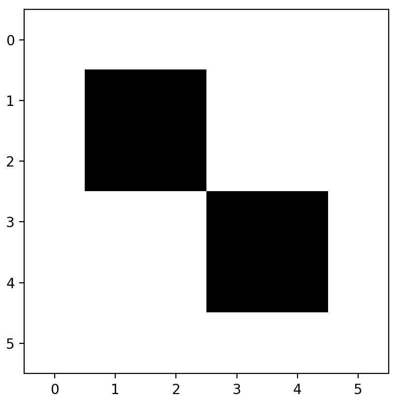
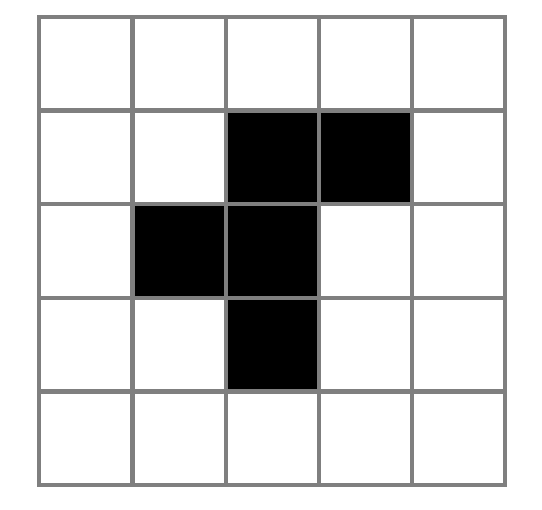
We must now decide on the seed. I will choose a simple oscillator, known as the beacon, which evolves as follows:
If you are struggling to see how this works, simply count the number of living neighbours for each cell then apply the rules of Life as presented earlier.
In python, we will set the seed like so:
beacon = [[1, 1, 0, 0],
          [1, 1, 0, 0],
          [0, 0, 1, 1],
          [0, 0, 1, 1]]

universe[1:5, 1:5] = beacon
It is worth discussing at this point how we plan on visualising our universe. The easiest solution I have come across is to use matplotlib’s imshow, which outputs a grid of colours corresponding to the value of every entry in an array. Using the binary colourmap, we have:
import matplotlib.pyplot as plt
plt.imshow(universe, cmap='binary')
plt.show()
3. Survival
We now need a function which will do the following:
- Take as arguments the x and y coordinates of a cell
- Examine the neighbours of this cell
- Decide whether the cell survives
- Write this into a new universe
The last point is rather subtle — we cannot update the cell in place, because this will affect the surrounding cells in the same iteration. Instead, we need to compute the survival of every cell based on a snapshot of the current universe, then simultaneously write all of these new cells into our universe. A cheap shortcut is to write the new values into a copy of the universe called new_universe, while leaving universe as a read-only. Then, later on, we can set the universe to be equal to new_universe.
# Create an identical copy of the universe, which will be the next generation.
new_universe = np.copy(universe)

def survival(x, y):
    """
    :param x: x coordinate of the cell
    :param y: y coordinate of the cell
    """
    # Find the number of living neighbours by taking
    # the sum of the 8 surrounding grid squares
    num_neighbours = np.sum(universe[x - 1:x + 2, y - 1:y + 2])
                     - universe[x, y]

    # If the cell is alive
    if universe[x, y] == 1:
        if num_neighbours < 2 or num_neighbours > 3:
            new_universe[x, y] = 0
    # Otherwise, the cell is dead...
    elif universe[x, y] == 0:
        # ... but it will rise again
        # IF there are three living neighbours
        if num_neighbours == 3:
            new_universe[x, y] = 1
I know that the if-else statements can be simplified drastically, like such:
if universe[x, y] and not 2 <= num_neighbours <= 3:
    new_universe[x, y] = 0
elif num_neighbours == 3:
    new_universe[x, y] = 1
But it is much more intuitive to keep the logic in its ‘expanded’ form, wherein one can clearly see the rules of Life.
4. Compute one full generation
This is a simple matter of applying our survival function to every cell in the universe, then setting universe to be equal to new_universe.
def generation():
    # We are inside a function, so we must specify
    # that we are referring to the global variable 'universe'.
    # Otherwise python will think that we are trying to
    # create a new variable also called 'universe'.
    global universe

    # Simple loop over every possible xy coordinate.
    for i in range(universe.shape[0]):
        for j in range(universe.shape[1]):
            survival(i, j)

    # Set universe to be equal to new_universe.
    universe = np.copy(new_universe)
5. Iterate and animate
There is no point iterating unless we can visualise the changes. To do so, we can simply use matplotlib’s animation module (see some examples here).
import matplotlib.animation as animation

fig = plt.figure()

# Remove the axes for aesthetics
plt.axis('off')
ims = []

for i in range(30):
    # Add a snapshot of the universe, then move to the next generation
    ims.append((plt.imshow(universe, cmap='Purples'),))
    generation()

# Create the animation
im_ani = animation.ArtistAnimation(fig, ims, interval=700,
repeat_delay=1000, blit=True)

# Optional to save the animation
im_ani.save('beacon.gif', writer="imagemagick")
Putting it all together, the output is:
Yes, I changed the colour to purple. Get over it.
Where here to go from here
In principle, we are done. Now it is up to you to experiment with different seeds! But I can’t resist one more demonstration, using the R-pentomino seed:
Perhaps you’d expect its behaviour to be vaguely similar to that of the beacon. But the wonderful thing about Life is the dazzling complexity that can result from a simple seed. See for yourself:
Check out my PyGameofLife repository on GitHub, which includes a slightly more professional refactoring with a number of built-in seeds allowing a user to generate gifs from the command line. The R-pentomino animation above can be created with:
python life.py -seed r_pentomino -n 500 -interval 50
Feel free to submit a pull request if you’d like to add more seeds or functionality.