Classifying financial time series using Discrete Fourier Transforms
A financial time series represents the collective decisions of many individual traders; it seems reasonable to me that the nature of these decisions may differ based on the underlying asset. For example, a company with a higher market cap may be more liquid, and subject to larger individual buy/sell orders including institutional investment. Thus, there is a case to be made that information such as the market cap of a company should be ‘encoded’ into its price movements. While these characteristics may be difficult to pinpoint on a chart, in principle it may be possible for a machine learning algorithm to find statistical relationships between the time series and the market cap of the company. This post will investigate that claim.
Concretely, a raw dataset will be constructed, consisting of 100-day price charts which belong to companies that are respectively in the top and bottom 1000 tickers in the Russell 3000 ordered by market cap. We will then run feature extraction (which is the core of this post), before applying a standard XGBoost classifier.
This post thus represents an intuitive (if naive) first approximation for classifying whether a given price chart belongs to a stock with high or low market cap. The hypothesis is that this problem is learnable, so the goal is to show that a machine learning model can classify a time series with greater than 50% accuracy. Though accuracy often has flaws as a metric, in this case it is sufficient because the classes will be almost perfectly balanced.
A discussion on classifying time series
Because much of real life data is temporal in nature, classifying and clustering time series has widespread importance, with such applications as:
- speech recognition
- medical data such as ECGs
- cyber-kinetic prosthetics: classifying electrical activity of muscles in terms of what action it corresponds to
- meteorological data
- seismic data
Some general approaches to classifying time series are as follows (a thorough survey can be found in Rani & Sikka 2012):
- Directly clustering with an algorithm like k-Nearest Neighbours. What is important here is a relevant distance metric between two different time series. Euclidean distance may not be sufficient as it has trouble dealing with timeseries that have been shifted slightly (either vertically or horizontally).
- Hidden Markov Models, which model the timeseries as a Markov Process, whose transition matrix may be used as input to a classifier.
- LSTM Neural Networks, which are fed in a time series and contain a sequential ‘memory’. The output of a cell can be run through the sigmoid function to convert it into a binary class value.
- Extracting summary statistics, then passing these results into a standard classifier.
This post will explore the last method. On the surface, it seems to be the most straightforward approach, but the difficulty is in choosing which aspects of the time series should be used. There are existing libraries that can extract a multitude of features, e.g. tsfresh, but although it is very likely that there is predictive power somewhere in here, it would be nice to find a simpler (and perhaps faster) approach.
Thus, I have decided to take the Discrete Fourier Transform (DFT) of the time series, and to use the largest terms as features. Such a method is really under the domain of spectral analysis, a well established subfield of time series analysis. However, we will adopt a rather informal approach. It should be noted that the Fourier Transform certainly shouldn’t be used to forecast the future of a financial time series because of the strong assumptions of periodicity. But it should be able to extract the main (sinusoidal) signals from a time series, which we can then put into a classifier.
Preparing the raw data
The data used in this project will be:
keystats.csv: parsed yahoo finance key statistics from which the latest market cap of securities will be ascertained. In order to reproduce something like this dataset (though only for the S&P500), please refer to my repo on GitHub- My
stock_pricesdatabase, which I discussed in this post.
After extracting the data from the csv files and MySQL database, I was left with a pandas dataframe sorted_tickers_by_mcap, containing tickers and their market caps, sorted by market cap in ascending order.
print("Number of tickers with mcap data available:",
       len(sorted_tickers_by_mcap))
print(sorted_tickers_by_mcap.head())
print(sorted_tickers_by_mcap.tail())
Number of tickers with mcap data available: 3382
Ticker
heat      67830.0
aryx     103730.0
gmet     336260.0
coco    1090000.0
dvox    1140000.0
Name: Market Cap, dtype: float64
Ticker
xom      3.632700e+11
msft     4.304200e+11
goog     4.942700e+11
googl    4.944500e+11
aapl     5.413300e+11
Name: Market Cap, dtype: float64
I then extracted the top and bottom 1000 tickers (removing the tickers for which data was not available), resulting in two lists of tickers: top_mcap and bottom_mcap:
Available top market cap: 831
Available bottom market cap: 862
These tickers are then sorted by market cap, and 100-day windows are made from the last 750 datapoints (roughly corresponds to 3 market-years). 3 years was chosen as the cutoff because market cap values from more than three years ago are likely to be significantly different from the latest values, as companies grow or shrink over time. A solution would be to use the keystats dataset to find the market cap for a company in a given year, but I have opted for a simpler workaround in this post.
Here is the function I wrote to create the time series snapshots from the raw price data.
def create_snapshots(ticker, n_days=750, window_size=100,
                     window_shift=50):
    """
    Returns list of time series of length windowsize, shifted
    by window_shift, for the last n_days.
    """
    df = pd.read_sql(f"SELECT adj_close_price FROM daily_price "
                    f"WHERE ticker_id={ticker_id[ticker]}", conn)
    df = df.iloc[-n_days:]
    snapshots = []
    for i in range(0, n_days, window_shift):
        window = df.iloc[i:i +window_size]
        window = window['adj_close_price'].values
        if len(window) == window_size:
            snapshots.append(window)
    return snapshots
These snapshots are then stacked into a numpy array as follows:
dataset = []

for i, ticker in enumerate(top_mcap):
    try:
        ticker_snapshots = create_snapshots(ticker)
    except Exception as e:
        print(str(e))
        continue
    ticker_snapshots = np.c_[np.array(ticker_snapshots),
                        np.ones(len(ticker_snapshots))]
    dataset.append(ticker_snapshots)

for i, ticker in enumerate(bottom_mcap):
    try:
        ticker_snapshots = create_snapshots(ticker)
    except Exception as e:
        print(str(e))
        continue
    ticker_snapshots = np.c_[np.array(ticker_snapshots),
                        np.zeros(len(ticker_snapshots))]
    dataset.append(ticker_snapshots)

dataset = np.vstack([a for a in dataset if a.shape[1] == 101])
The first 10 rows of dataset are presented below. Note how the last column is always 1 – this is because the first half of the dataset consists of the top market cap tickers (classified as 1).
array([[35.639999, 35.610001, 39.220001, ..., 37.189999, 37.060001,
         1.      ],
       [40.369999, 40.369999, 40.419998, ..., 36.189999, 35.889999,
         1.      ],
       [37.810001, 37.849998, 38.419998, ..., 34.68    , 34.959999,
         1.      ],
       ...,
       [41.369999, 40.02    , 39.860001, ..., 35.279999, 35.27    ,
         1.      ],
       [38.5     , 38.669998, 38.599998, ..., 41.169998, 41.27    ,
         1.      ],
       [35.360001, 35.439999, 36.34    , ..., 42.740002, 43.349998,
         1.      ]])
We have now finished preparing the raw data for analysis. However, we still need to extract the features and preprocess the data for machine learning specifically. This will be covered in the next section.
Methodology
It is a remarkable fact of mathematics that periodic functions (at least the well-behaved ones) can be decomposed into sines and cosines. Although price data certainly isn’t periodic, if we treat the whole time series as one period, we can apply a Discrete Fourier Transform (DFT) to extract the main ‘signals’ in a time series. My motivation for using a DFT is that it can be used to de-noise a time series by ignoring the smaller terms, and that the coefficients of the resulting terms can be fed into a classifier. Additionally, there exist very efficient implementations in numpy, such as np.fft.fft(). One potential problem is that the results of the DFT are actually complex numbers:
array([ 3.86450001e+02+0.j        , -7.77637336e+00+2.22326054j,
       -3.85445493e+00+2.69405956j, -2.39862764e+00+4.72442769j,
       -1.07054807e+00+1.46787384j,  1.49997000e-01+0.j        ,
       -1.07054807e+00-1.46787384j, -2.39862764e+00-4.72442769j,
       -3.85445493e+00-2.69405956j, -7.77637336e+00-2.22326054j])
This begs the question as to how we can input the DFT terms into a classifier. We will implement and compare two possible methods.
- Taking the modulus (
np.abs) of each term and using that as a feature - Splitting up the real and imaginary parts to use as separate features.
Clearly, we would expect the latter to have more predictive power, but at the cost of using twice as many terms.
There is another decision we have to make, namely, how many terms of the DFT we want to use. As it is impossible to know a priori how much information the Fourier terms hold, we’ll examine the first 5, 15, and 30 terms.
So in total, we have 6 datasets to test. Now, in order to avoid the data mining bias, we will apply a Bonferroni correction. The idea is that each additional test increases our chance of finding a spurious yet statistically significant relationship, so to counteract this, the significance level must be decreased to $\frac{\alpha}{m}$, where $m$ is the number of tests. So if the original significance level was $\alpha = 0.05$, the Bonferroni correction would imply a new significance of $\frac{\alpha}{6} = 0.00833$.
Feature extraction and data preprocessing
Adopting standard scikit-learn notation, X will denote the feature array and y the target vector. Using the dataset that we prepared before:
X = dataset[:,:-1]
y = dataset[:, -1]
Prior to putting our data through a DFT, I am first going to standardise the time series (scale everything to the range [0,1]) to ensure that we don’t actually learn some boring correlation between the share price of a company and its market cap. To maximise the efficiency of this computation, bearing in mind that this computation needs to be done for more than 20k rows, it is important to (ab)use numpy’s broadcasting:
numerator = X - X.min(axis=1).reshape((len(X), 1))
denominator = X.max(axis=1) - X.min(axis=1)
denominator = denominator.reshape((len(X),1))
X_scaled = numerator/denominator
We will now define functions to take the Fourier Transform, then slice for the first k terms, before either taking the modulus or splitting into real and imaginary parts.
def generate_modulus_dataset(X, k):
    return np.abs(np.fft.fft(X)[:, :k])

def generate_complex_dataset(X, k):
    fourier = np.fft.fft(X)[:, :k]
    return np.column_stack((fourier.real, fourier.imag))
With these methods ready, creating all of the datasets is simple:
modulus_5 = generate_modulus_dataset(X_scaled, 5)
modulus_15 = generate_modulus_dataset(X_scaled, 15)
modulus_30 = generate_modulus_dataset(X_scaled, 30)
complex_5 = generate_complex_dataset(X_scaled, 5)
complex_15 = generate_complex_dataset(X_scaled, 15)
complex_30 = generate_complex_dataset(X_scaled, 30)
Machine Learning
We are finally ready to apply machine learning using python’s wonderfully intuitive sklearn. I have chosen to use an XGBoost classifier – it trains quickly and normally produces good results with the default parameters. It should be noted that no hyperparameter optimisation will be done: the point of this experiment is to see if this problem is learnable (rather than trying to achieve excellent results). I have written the classification script as a function which can be easily applied to each of the datasets.
from sklearn.model_selection import train_test_split
from xgboost import XGBClassifier
from sklearn.metrics import precision_score, accuracy_score


def classify(features, target, return_acc=False):
    X_train, X_test, y_train, y_test = train_test_split(
                                            features, target)
    clf = XGBClassifier()
    clf.fit(X_train, y_train)
    y_pred = clf.predict(X_test)

    acc = accuracy_score(y_test, y_pred)
    prec = precision_score(y_test, y_pred)
    if return_acc:
        return acc
    print(f"Accuracy:\n {100* acc:.2f}%")
    print(f"Precision:\n {100* prec:.2f}%")
It is then a simple matter of applying the function to any of our datasets:
classify(modulus_5, y)
Running the above resulted in a cross-validated accuracy of 58%. Given balanced classes, this is clearly a significant difference, so in principle the experiment could be stopped here and we can conclude that classifying stock charts based on market cap is a learnable problem. This result was especially surprising to me because this particular example is just using the moduli of the first 5 terms of the Fourier Transform, which really ignores a lot of the price chart. To see what I’m talking about, this is what a time series made of the absolute values of the first 5 Fourier terms looks like:
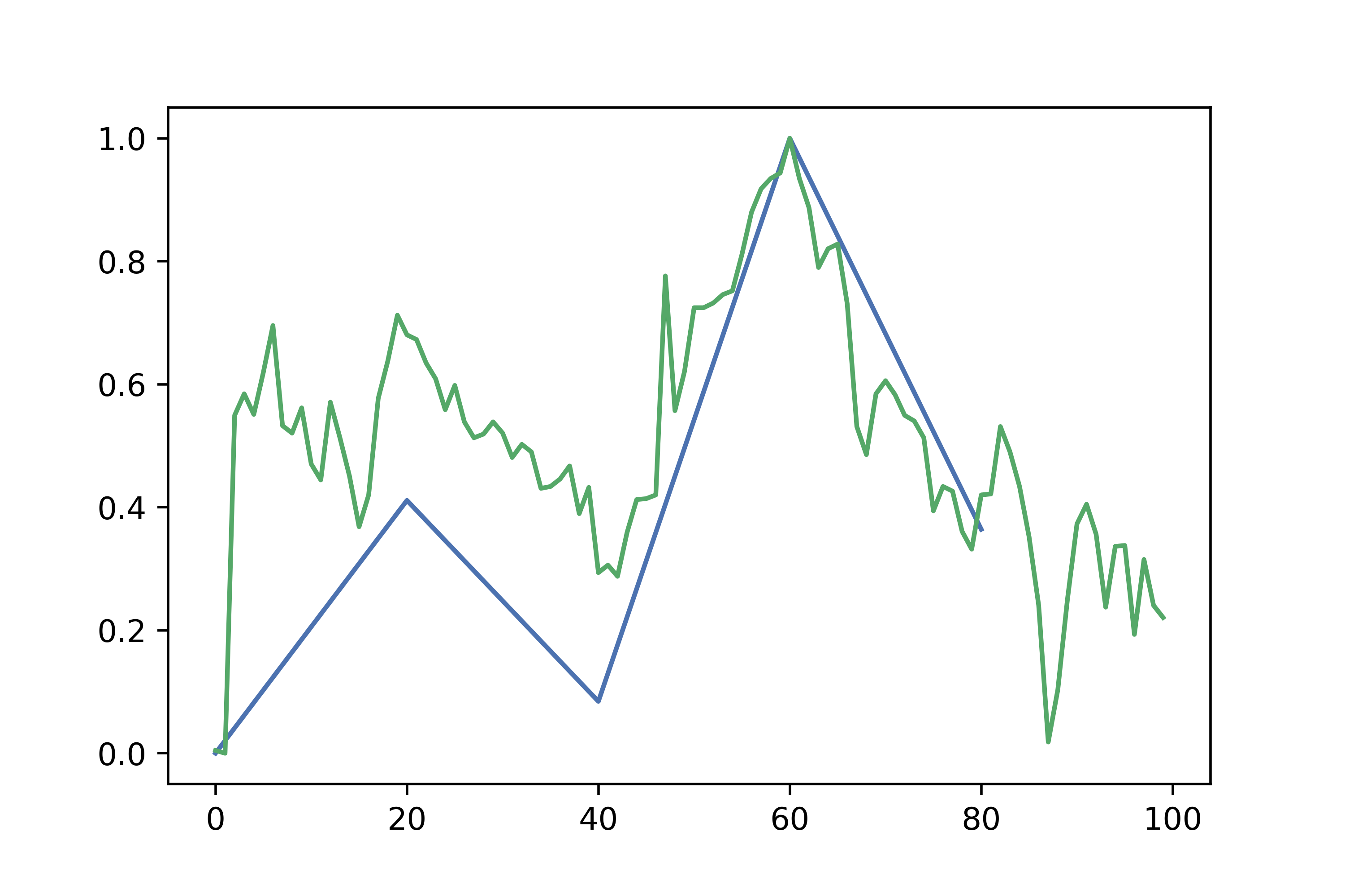
Although you can see that some of the main trends are captured, it is clearly a crude approximation that ignores a lot of variation.
Despite having achieved our initial goal of demonstrating the learnability of this problem, seeing as we have already prepared the datasets it may be interesting to do further analysis.
Comparison with a benchmark
What happens if we try to naively classify based on the whole time series, i.e using each of the 100 days’ prices as a feature?
%%time
classify(X_scaled, y)
Accuracy:
 65.34%
Precision:
 64.48%
CPU times: user 18.6 s, sys: 135 ms, total: 18.7 s
Wall time: 19.2 s
So actually the naive benchmark has a much better accuracy. But note the relatively long compute time of 18.7s. The question is whether any of our other datasets can reach comparable accuracies more efficiently.
%%time
classify(complex_5, y)
Accuracy:
 60.96%
Precision:
 60.17%
CPU times: user 1.96 s, sys: 18.5 ms, total: 1.97 s
Wall time: 2.04 s
It makes sense that the complex dataset has a higher accuracy than the modulus dataset for the same number of Fourier terms: bear in mind that it includes twice as many features (since we have split the real and imaginary part).
%%time
classify(modulus_15, y)
Accuracy:
 59.45%
Precision:
 57.72%
CPU times: user 3.77 s, sys: 62.8 ms, total: 3.83 s
Wall time: 4.33 s
This is an interesting result. 15 modulus terms (15 features) underperform 5 complex terms (i.e 10 features). This tells us that the actual complex number holds a lot of information.
%%time
classify(complex_15, y)
Accuracy:
 64.97%
Precision:
 63.75%
CPU times: user 3.02 s, sys: 26.1 ms, total: 3.04 s
Wall time: 3.09 s
Using 15 complex terms (i.e 30 total features), comparable accuracy to the benchmark has been achieved, in about a sixth of the time!
%%time
classify(modulus_30, y)
Accuracy:
 59.74%
Precision:
 57.98%
CPU times: user 3.16 s, sys: 35.1 ms, total: 3.19 s
Wall time: 3.33 s
%%time
classify(complex_30, y)
Accuracy:
 66.63%
Precision:
 65.24%
CPU times: user 11.9 s, sys: 136 ms, total: 12.1 s
Wall time: 12.6 s
We can observe the diminishing returns: using more Fourier terms increases accuracy only slightly. However, it is a pretty remarkable result that using 30 complex terms (i.e 60 features), we can beat the benchmark while also being 1.5x faster.
To better visualise how accuracy varies with the number of terms, we can generate multiple datasets and run our classification method on them:
scores = []
for i in range(0, 100, 5):
    print(i)
    dataset = generate_modulus_dataset(X_scaled, i)
    acc = classify(dataset, y, return_acc=True)
    scores.append(acc)
Doing the same for the complex datasets and plotting the results yields:
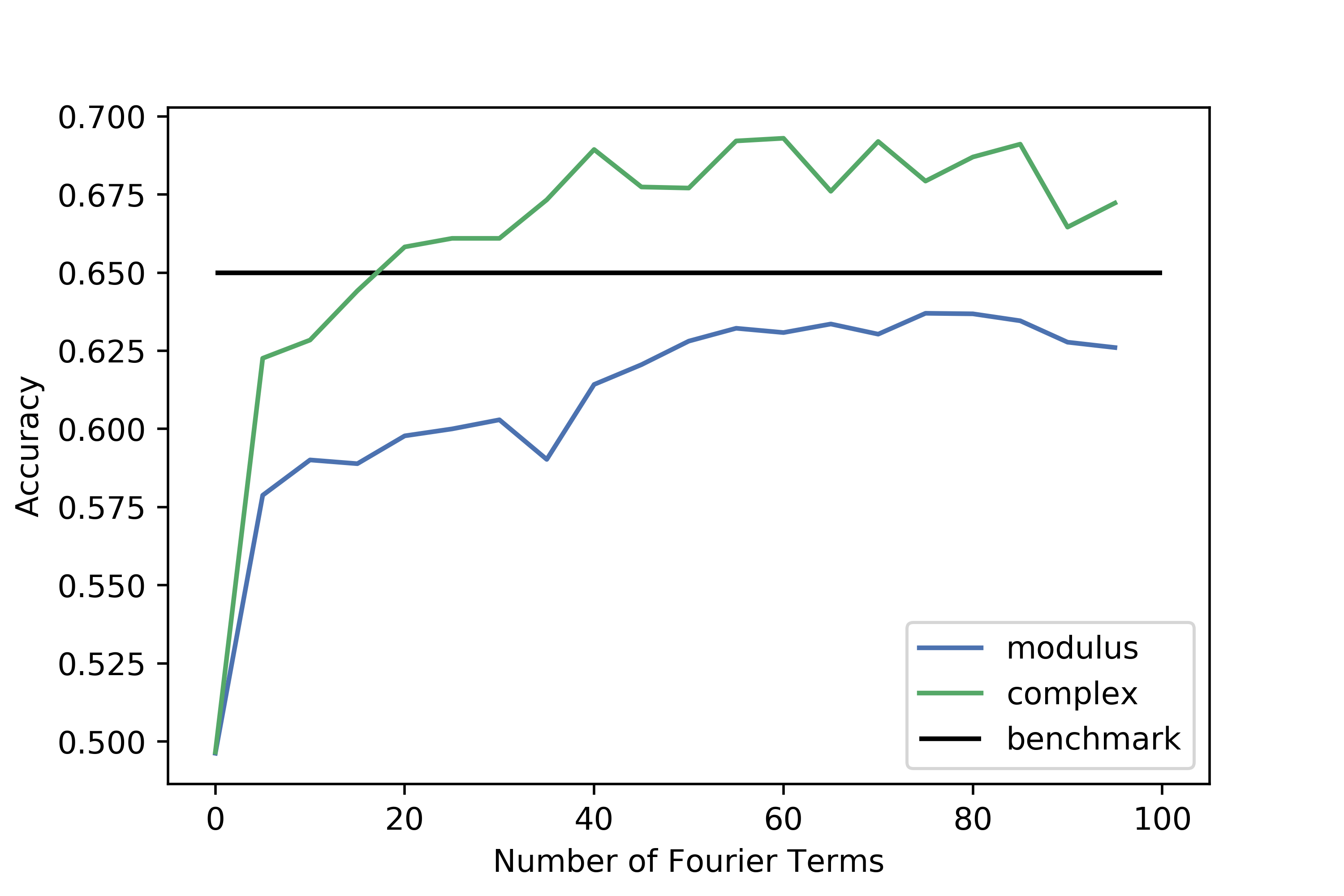
It is interesting to note that the modulus datasets never beat the benchmark: it seems that taking the modulus of the complex terms throws away too much information. The complex datasets are most predictive at around 40 terms, but the plateau and gradual decrease after that is a clear sign that overfitting occurs.
Conclusion
In this post, we have seen that we can determine whether a given 100-day time series of stock prices belongs to a high market cap or low market cap stock, with more than 65% accuracy. This was done by extracting the main signals from a time series with a Discrete Fourier Transform, which were then used as features in a classifier. The DFT is not only able to outperform the naive solution of using each day’s price as a feature, but can also do so with a large speedup. The implication of this is that the benchmark overfits to noise, and thus this is a practical example of how reducing the information available to a classifier can actually improve performance.
I think this is an important lesson for anyone applying machine learning to a real-world problem: throwing data at a classifier or deep learning model is not a solid approach. First try to extract important features or at least discard those that only contribute noise.
Future work on this topic could involve comparing the classification performance of the DFT method to a classifier that uses different summary statistics, or perhaps even a clustering methodology like k-Nearest Neighbours. But for now I am satisfied that this simple and intuitive method is sufficient to do significantly better than random guessing.