Graph algorithms and currency arbitrage, part 1

Arbitrage is the holy grail for traders and the bedrock of financial academia. Let’s say you are in an open marketplace with Alice selling oranges for \$1 each and Bob buying them for \$2. As a cunning trader, you realise you can buy an orange from Alice and immediately sell it to Bob for \$1 of “risk-free” profit. However, as you keep reaping this \$1 profit by buying up Alice’s oranges, she raises her prices. Eventually, Alice would be charging \$2 per orange and the arbitrage would be shut. In other words, acting on arbitrage opportunities causes the market to become more efficient, with everything as close to its fair price as possible. Because of this, the only way to profit from true arbitrage is to find and execute opportunities faster than everybody else.

Currency exchange is a natural place to search for arbitrage because there are many different pairs that we can trade. For example, assume we are able to convert GBP to USD, then USD to EUR, then EUR to AUD for an effective rate of 1:2 GBP:AUD. If we were then able to directly swap AUD back to GBP in the ratio 2:1.1, this would be an arbitrage opportunity because we end up with more GBP than we started with while taking zero risk.

Our goal is to develop a systematic method for detecting arbitrage opportunities by framing the problem in the language of graphs. This is a reasonably large topic, so we’ll split it into two parts. Part 1 (this post) will lay the theoretical groundwork, introducing graph algorithms and giving an overview of their application to currency arbitrage. In Part 2 we will present an actual implementation of these ideas in python, applied to cryptocurrencies.

Graphs

Formally, we define a graph as a set of vertices (also called nodes) and edges. These edges can be directed (i.e have little arrows on them) and may have weights. It is completely up to us to decide what the vertices, edges, and weights represent. For example, if we are trying to model a road network we might say that the vertices are cities (or junctions), the edges are the roads themselves, and the weights are the length of the roads. The diagram below shows how a weighted directed graph is typically depicted.

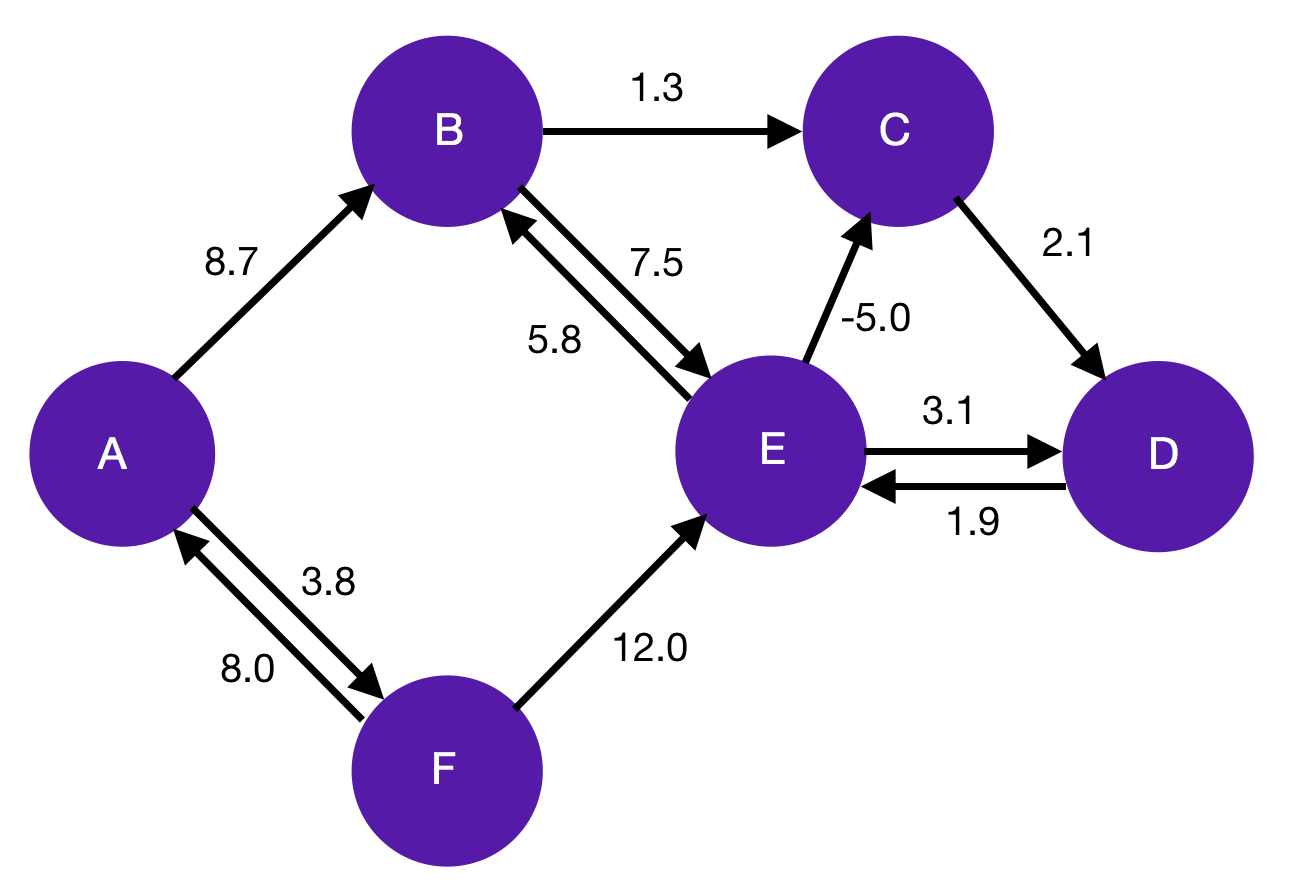
It is useful to formulate real-world problems in terms of graphs because we have about three centuries worth of relevant theory – they were first investigated by Euler in 1736. In particular, there exist many efficient algorithms related to finding the shortest path along a graph, which have widespread applications e.g. in mapping.

The Bellman-Ford algorithm finds the minimum weight path from a single source vertex to all other vertices on a weighted directed graph. For the purposes of this post, we don’t need to know anything other than the fact that once the algorithm terminates, each vertex is labelled with the total weight of the minimum weight path from the source to that vertex.

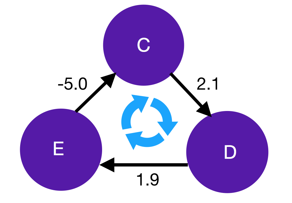
Actually, the above statement has an incredibly important caveat. What happens if we try to find the minimum weight path from vertices C to D in the above graph? The obvious guess would be that it is the direct path along the CD edge, which has total weight 2.1. However, notice that we can in fact reduce this further by following the path CDECD, which would have a total weight of -1. But why stop there? If we go around the loop again, we can reduce it stil further. In fact, each time we traverse the loop, our minimum total weight will reduce by 1. Hence this is called a negative-weight cycle, the existence of which means that the shortest path between C and D is not defined.

This is actually the main reason why we are choosing to use Bellman-Ford over another shortest path algorithm like Dijkstra, despite the latter being asymptotically more efficient. Bellman-Ford is able to detect if there is a negative-weight cycle and as will be seen shortly, this will be the key to detecting arbitrage opportunities.

Graphs for currency arbitrage

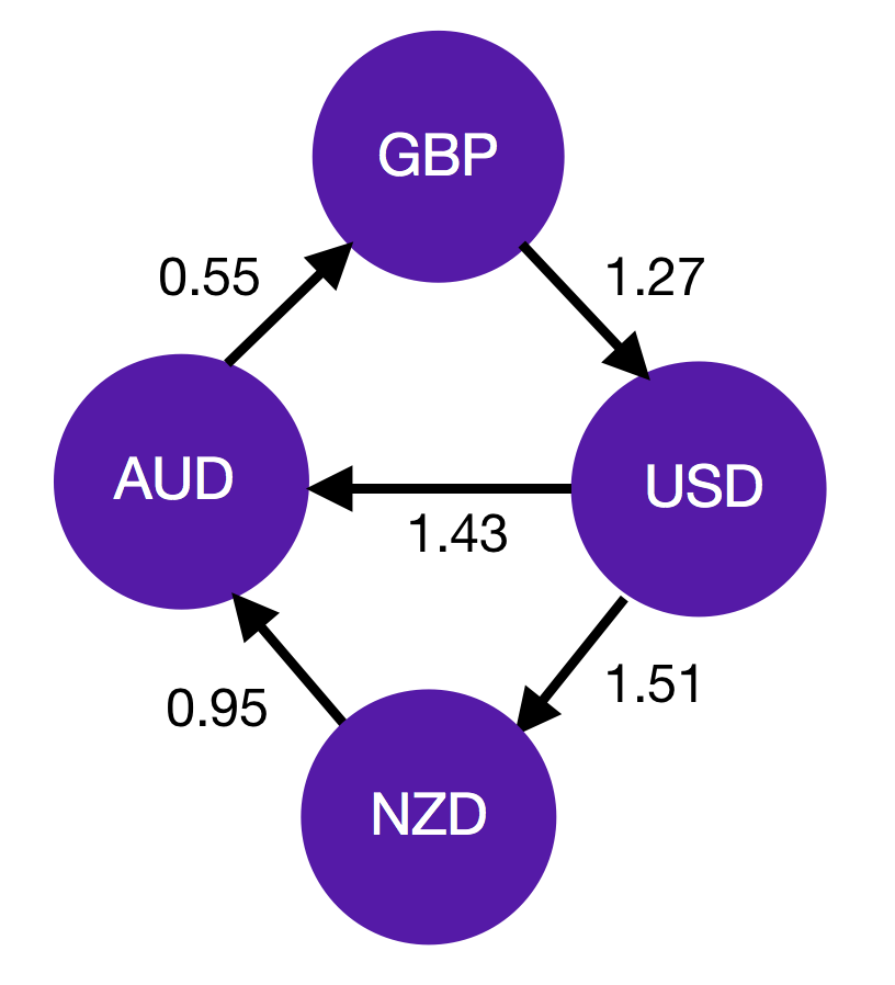
How can graphs be used to model currency markets? At a very high level, we will assign currencies to different vertices, and let the edge weight represent the exchange rate. A simple example is presented below: in this market, we can convert 1 GBP to 1.27 USD, 1 USD to 1.43 AUD, etc.

To find the exchange rate between two currencies that do not share an edge, we simply find a path between the two currency vertices and walk along it, multiplying by each successive edge weight (exchange rate). If there are multiple possible paths, choose the path that has the greatest weight product, which corresponds to the most favourable rate.

What would happen if we start with 1 GBP and convert it along GBP $\to$ USD $\to$ AUD $\to$ GBP? Well, multiplying out the edges we see that our initial 1 GBP becomes $1.27 \times 1.43 \times 0.55 \approx 0.999$ GBP. That is to say, we lose a tenth of a penny on the round trip. However, if this number were greater than 1, it would mean that by following this path we end up with more GBP than we started with – this is textbook arbitrage.

So the problem of finding arbitrage can thus be formally posed as follows: find a cycle in the graph such that multiplying all the edge weights along that cycle results in a value greater than 1. In fact we have already described an algorithm that can find such a path – the problem is equivalent to finding a negative-weight cycle, provided we do some preprocessing on the edges.

Firstly, we note that Bellman-Ford computes the path weight by adding the individual edge weights. To make this work for exchange rates, which are multiplicative, an elegant fix is to first take the logs of all the edge weights. Thus when we sum edge weights along a path we are actually multiplying exchange rates – we can recover the multiplied quantity by exponentiating the sum. Secondly, Bellman-Ford attempts to find minimum weight paths and negative edge cycles, whereas our arbitrage problem is about maximising the amount of currency received. Thus as a simple modification, we must also make our log weights negative.

With these two tricks in hand, we are able to apply Bellman-Ford. The minimal weight between two currency vertices corresponds to the optimal exchange rate, the value of which can be found by by exponentiating the negative sum of weights along the path. As a corollary, we have the wonderful insight that: a negative-weight cycle on the negative-log graph corresponds to an arbitrage opportunity.

Conclusion

We have seen that graphs provide an elegant framework for thinking about currency exchange. Concretely, by representing different currencies as vertices and using the negative log of the exchange rate as the edge weight we can apply shortest-path algorithms to find negative-weight cycles if they exist, which correspond to arbitrage opportunities. In the next post, we code up the methodology presented in this post and apply it to some real-world data. Should be fun!