How predictive is the historical volatility?

One of the things that makes markets exciting (or frightening) is that prices move around a lot. It is important to be able to describe and predict the range of possible price movements over a given time horizon since some investors might desire assets whose prices don’t move up and down too much. We can quantify this by computing the volatility, which is commonly defined to be the standard deviation of the asset’s (log) returns. This post examines how well we can predict future volatility and why that matters.

Volatility is a rather important quantity because it is the default way for investors to quickly assess the amount of risk that a stock might add to the portfolio. It also shows up in many different parts of finance, from the traditional Capital Asset Pricing Model used in investment banking to option-pricing. One of the most tangible applications, however, is in portfolio optimisation, which attempts to constructs portfolios that meet certain investor objectives, for example, finding the that minimises the total volatility. The general procedure for doing this is to estimate the future returns and covariance of a group of stocks (normally basing these estimates on historical values) then running an optimisation procedure – I have written about this extensively in the documentation for my portfolio optimisation software library.

However, the key to this procedure is that we are assuming that the past is a reasonable predictor of the future. A large amount of research has shown that historical returns are a very poor predictor of future returns, but I haven’t seen many comments on whether historical volatility is a good predictor of future volatility. This post is a brief investigation into the matter.

Methodology and hypothesis

We are going to keep this post extremely simple and examine the predictability of the S&P500’s volatility. Firstly, we will collect adjusted closing prices for the S&P500 over a large timeframe. We will then form 1y, 3y, 5y, 10y, 20y rolling windows and compute the rolling volatility for each. These will then be correlated with the realised volatility.

The reason for this is that I am quite interested to know how much data is required to make a better estimate of future volatility. My hypothesis is that there will be some intermediate optimum – too little data and you can’t make a good estimate, but too much data dilutes recent datapoints with ancient ones (which may be less relevant).

Preparing data

We start by using pandas_datareader to acquire some free price data from Yahoo Finance. Remarkably, we can get daily OHLCV (open, high, low, close, volume) data all the way back to 1927. I am of the opinion that it is good practice to save whatever data you download to the disk, in case you need it later.

import pandas as pd
from pandas_datareader import data as web

sp500_df = web.DataReader("^GSPC", "yahoo", 
                          datetime.datetime(1950,1,1), 
                          datetime.datetime(2019,12,19))
sp500_df.to_csv("data/sp500_prices.csv")

We can then read the data back in and clean it up. In particular, for this exploration we only need the Adj Close column, which contains the daily close prices adjusted for dividends and stock splits.

sp500_df = pd.read_csv("data/sp500_prices.csv", parse_dates=True)
px = sp500_df.set_index("Date")["Adj Close"]

It is straightforward to compute returns thanks to the pct_change() methods, which calculates the percentage change between dataframe rows.

rets = px.pct_change().dropna()
rets.head()

Date
1950-01-04    0.011405
1950-01-05    0.004748
1950-01-06    0.002953
1950-01-09    0.005889
1950-01-10   -0.002927
Name: Adj Close, dtype: float64

Because the price data excludes weekends and holidays, a trading year is actually only 252 days. To calculate the rolling volatility for a given window, we can just rely on the magic of pandas:

import numpy as np

rolling_vol = rets.rolling(time_period * n_days).std() * np.sqrt(252)

The np.sqrt(252) arises because volatilities are most commonly expressed on annual terms, whereas the method calculates a daily volatility. Combining all of this into a loop so that we can easily repeat the calculation for multiple time periods:

n_days = 252  # trading days in a year
time_periods = [1, 3, 5, 10, 20]  # in years
stds = []
for t in time_periods:
    stds.append(rets.rolling(t * n_days).std())
std_df = pd.concat(stds, axis=1)
std_df.columns = [f"{t}y" for t in time_periods]
std_df *= np.sqrt(252)  # annualise

The result of this is a dataframe where each column represents a different window length.

Date		1y	        ...     20y			
2019-12-13	0.143483	...     0.188674
2019-12-16	0.142234	...     0.188642
2019-12-17	0.140569	...     0.188635
2019-12-18	0.140573	...     0.188622
2019-12-19	0.139656	...     0.188622

Having now computed our historical volatility estimates, we need to calculate the realised volatilities (this is what we are trying to predict). This can be done with a nice pandas trick, using the shift() method to “look into the future”:

# Compute realised annual volatilities
realised_vol = rets.rolling(n_days).std().shift(-n_days) * np.sqrt(252)
realised_vol = realised_vol.rename("realised_vol")
realised_vol.head()

Date
1950-01-04    0.148951
1950-01-05    0.148979
1950-01-06    0.149594
1950-01-09    0.150306
1950-01-10    0.150330
Name: realised_vol, dtype: float64

Having collected and processed the data, we are now ready to conduct an analysis.

Analysis

Firstly, let’s plot all of the rolling volatilities that we calculated.

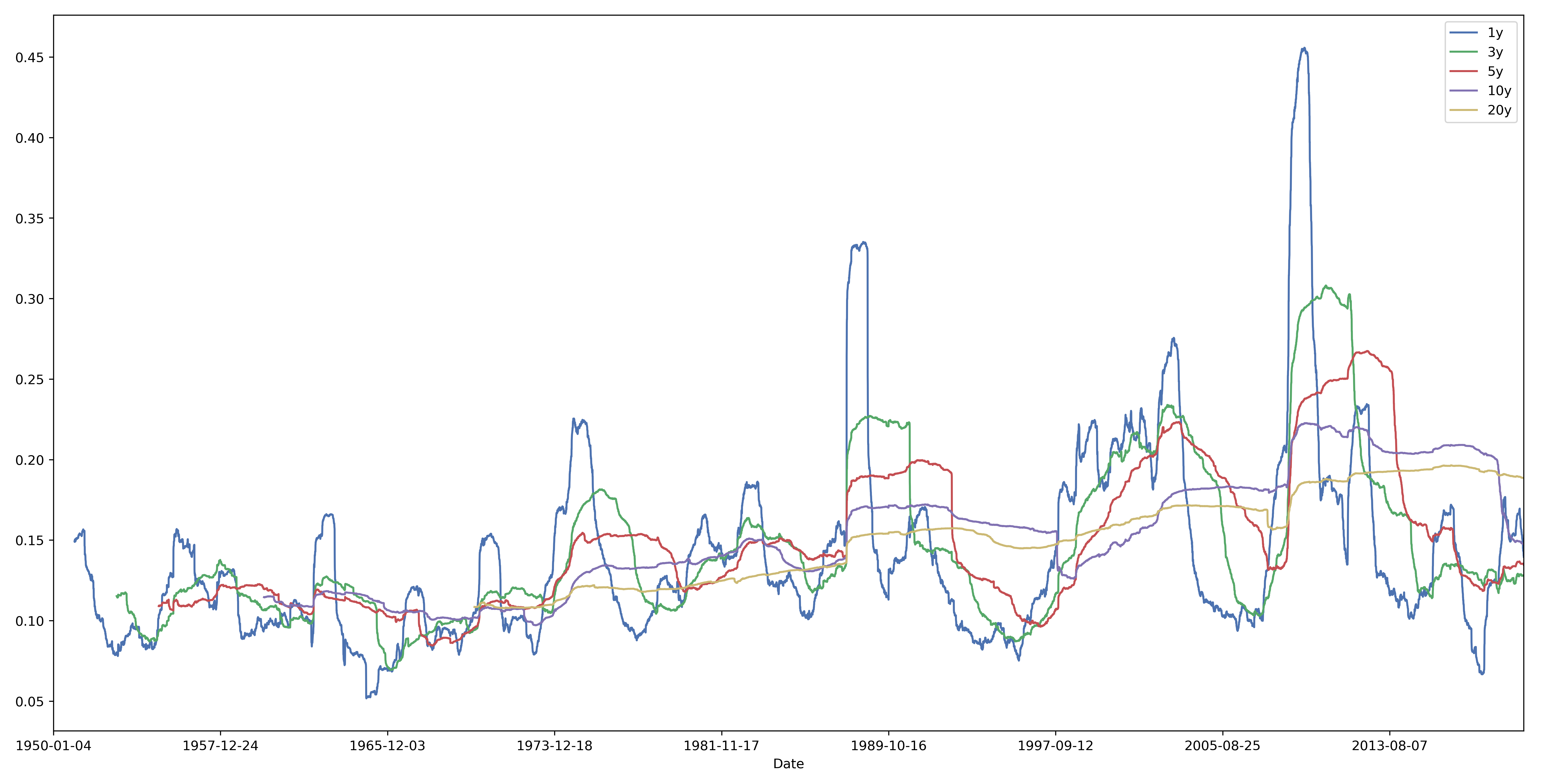
Clearly, the wider the rolling window, the more stable our estimate of volatility. This is reflected in the fact that the yellow line moves around much less than the blue line, which exhibits many spikes. On the subject of spikes, it is interesting to note that the spikes seem to correspond to market crises: 2008 MBS, 2002-03 DotCom, 1987 Black Monday, 1973-74 oil crisis, and the 1962 Kennedy Slide (along with many other smaller ones). I find it equally interesting that most of the volatility spikes are extremely short-lived, which suggests to me that markets don’t take too long to re-price assets following a major shift.

But that is almost a tangent – the main point of this post is to understand how the historical volatility correlates with future realised volatility. The correlation coefficients are as follows:

std_df.corrwith(realised_vol)

1y     0.429631
3y     0.286037
5y     0.176046
10y    0.179328
20y    0.058464

These results are quite shocking. Firstly, I find the overall trend to be surprising, as I expected either the 3y or 5y to strike the right balance between recency and stability. It is quite surprising that using only the last year’s volatility to estimate future volatility has the most predictive power, but there you go. Secondly, the actual values are quite low. To put it differently, even for the 1y data, historical volatility only explains 18% ($0.4296^2$) of the variance in the realised volatility.

However, the explained variance is often not as intuitive as you might expect. I believe that a more tangible number is the Mean Absolute Error (MAE), which tells us how far away our prediction is from the realised volatility, on average.

mae = np.abs(std_df.subtract(realised_vol, axis=0)).mean()

1y     0.043003
3y     0.048608
5y     0.050167
10y    0.050909
20y    0.049677

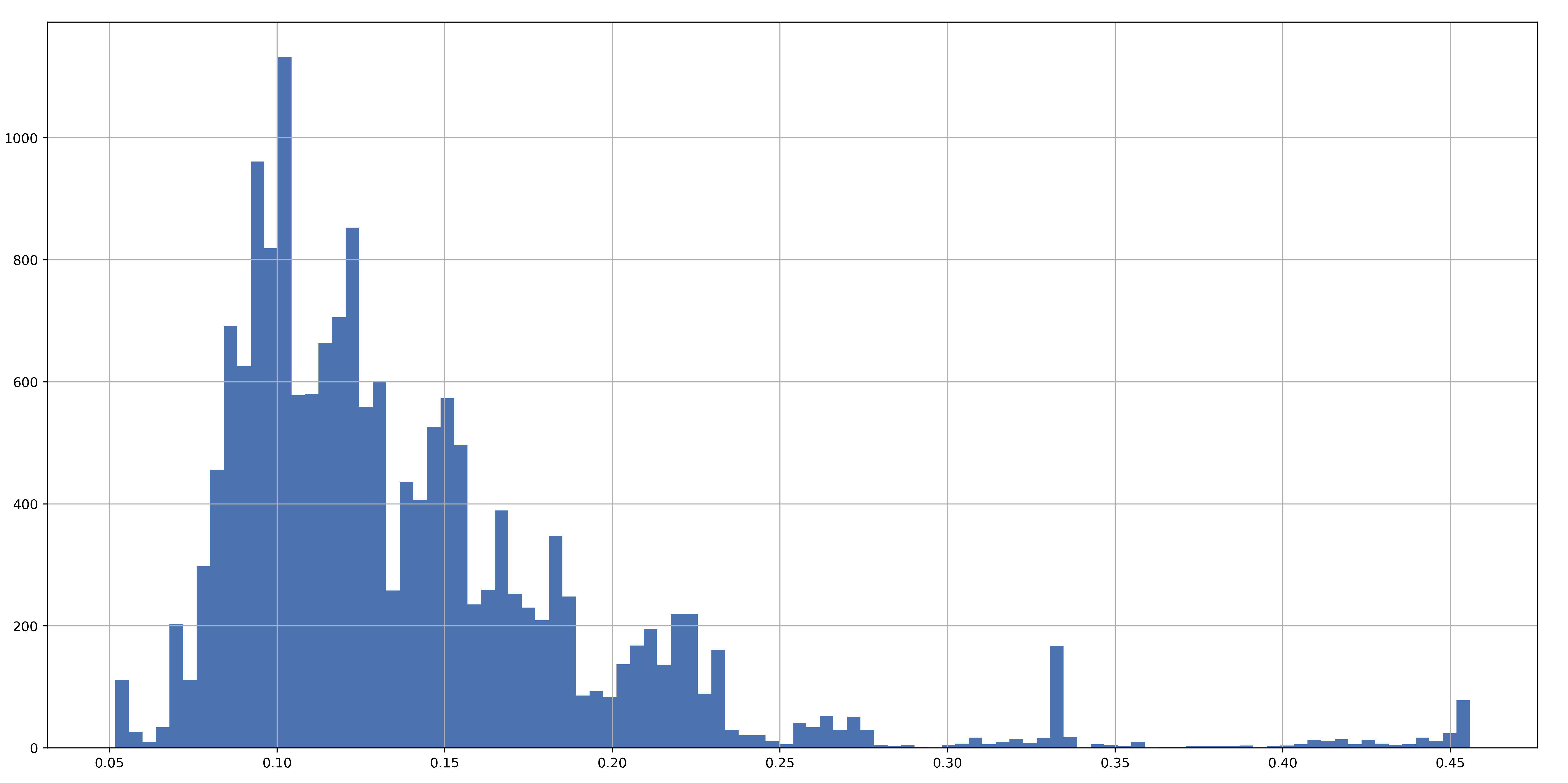
For the 1y data, historical volatility had a MAE of about 4.3%, which is quite large! However, looking through the data I saw that it was a few far-off predictions that caused such awful results. This is corroborated by a histogram of the realised volatilities, for which we can observe a fat right tail:

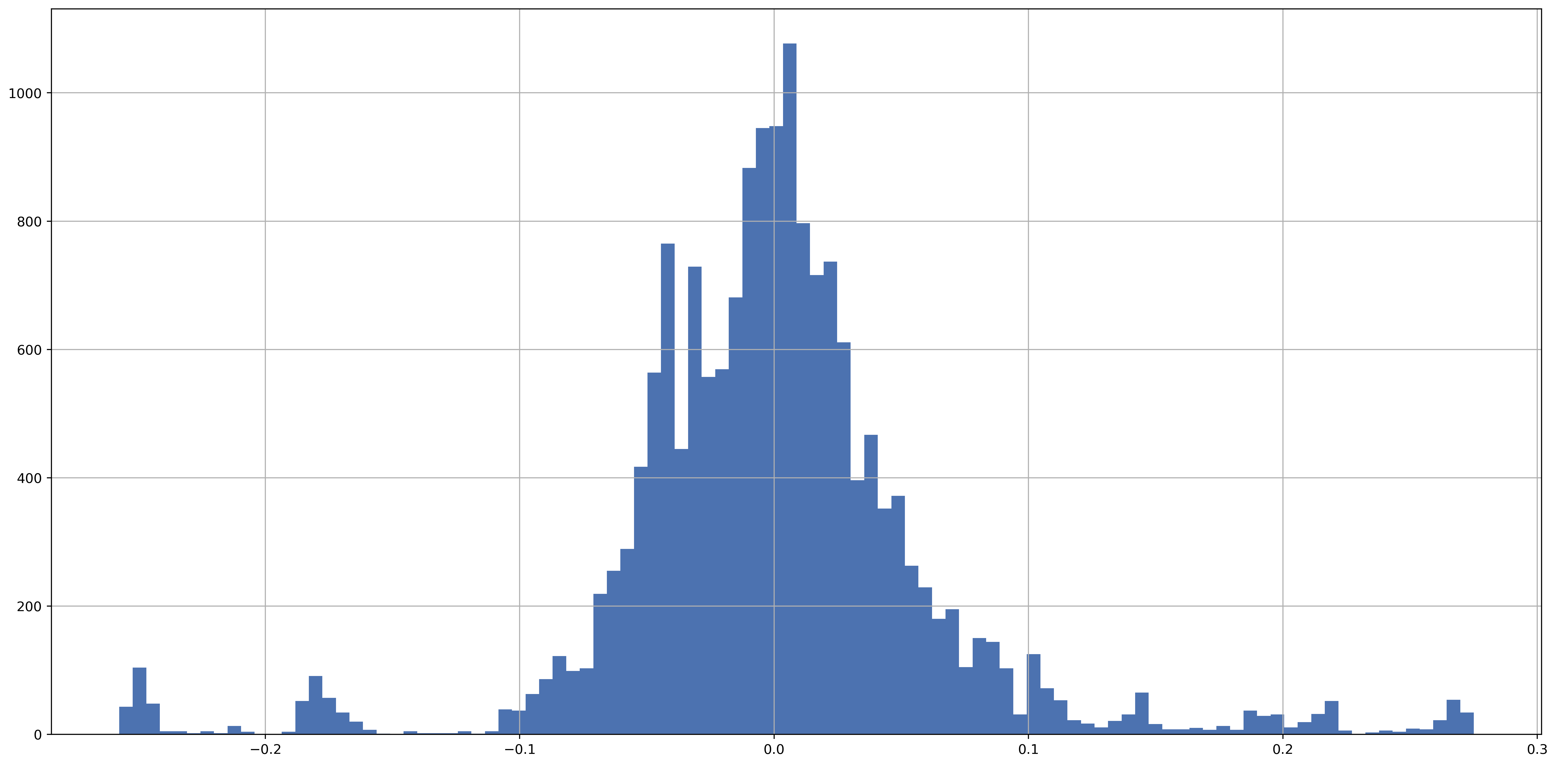
All of these findings notwithstanding, it is reassuring to see that the errors between historical and realised volatilities are almost centred around zero:

(std_df["1y"] - realised_vol).hist(bins=100)

Conclusion

In conclusion, we see that historical volatility is far from a perfect forecaster of future volatility, explaining less than 20% of the variance in realised volatilities in the best case (out of our experiments). It is not entirely surprising that this is the case, given that volatility forecasting is a very heavily-researched topic, since a better estimate of the volatility gives you a competitive advantage when it comes to pricing options or trading volatility instruments like the VIX. There are numerous sophisticated econometric models for predicting future volatility, not least the GARCH family, so it is naive to assume that simply using the historical volatility would give good results.

When it comes to the topic of portfolio optimisation, these findings should be a real wake-up call that you need to consider the uncertainties in both your return estimates and volatility/covariance estimates. It is true that the mean-variance machinery is not able to take this into account – all the more reason to swap to a confidence-aware Bayesian method such as Black-Litterman optimisation. However, even then, it is not straightforward to understand the potential effects of the skewed distribution of realised volatilities.

It should be noted that not everyone agrees that the volatility is a number worth paying attention to in the first place. A famous critic is Warren Buffet, who rightly points out that a good company whose stock price suddenly drops due to temporary factors (e.g. a media scandal) could be a bargain purchase – in which case it is actually less risky than it was before, although its volatility will be higher as a result of the drop. Perhaps this post lends some evidence to this point of view. Given the distribution of realised volatilities, it seems that the converse may also be true: even if everything looks calm and you predict low volatility, a right-tail event could make things go horribly wrong. As is always the case in finance, caveat emptor applies!

The full Jupyter notebook can be found on my GitHub